■ はじめに
Kaggle初心者向けのコンペに取り組みましたので
簡単にまとめてみました。
【概要】
・Titanic: Machine Learning from Disaster
・沈没する船「タイタニック号」の乗客情報をもとに、助かる人とそうでない人について判別する
今回はロジスティック回帰を用いて、モデルの作成をしていきます。
1. モジュールの用意
import numpy as np
import pandas as pd
import matplotlib.pyplot as plt
import seaborn as sns

from sklearn.preprocessing import StandardScaler
from sklearn.model_selection import train_test_split
from sklearn.linear_model import LogisticRegression
from sklearn.metrics import roc_curve, roc_auc_score
from sklearn.metrics import accuracy_score, f1_score
from sklearn.metrics import confusion_matrix, classification_report
from sklearn.feature_selection import RFE

%matplotlib inline
## 2. データの準備
train = pd.read_csv('train.csv')
test = pd.read_csv('test.csv')

print(train.shape)
print(test.shape)

# (891, 12)
# (418, 11)
train.head()
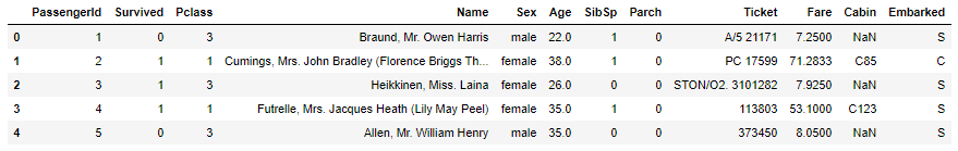
【データ項目】
・PassengerId:乗客ID
・Survived:生存したかどうか(0:助からない、1:助かる)
・Pclass – チケットのクラス(1:上層クラス、2:中級クラス、3:下層クラス)
・Name:乗客の名前
・Sex:性別
・Age:年齢
・SibSp:船に同乗している兄弟・配偶者の数
・parch:船に同乗している親・子供の数
・ticket:チケット番号
・fare:料金
・cabin:客室番号
・Embarked:船に乗った港(C:Cherbourg、Q:Queenstown、S:Southampton)
test.head()
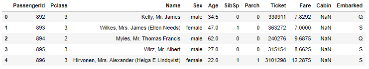
testデータの乗客番号(PassengerId)を保存しておきます。
PassengerId = test['PassengerId']
実際にはtrainデータのみでモデルの作成を行いますが
モデルにtestデータを投入する際、同じ特徴量が必要となります。
前処理にOne-Hot-Encodingなどを使用した場合、
trainとtestデータの特徴量数が異なってしまうため
両データを結合し、まとめて前処理を行っていきます。
まず、trainデータは項目が1つ多い(目的変数:Survived)ので分離します。
y = train['Survived']
train = train[[col for col in train.columns if col != 'Survived']]

print(train.shape)
print(test.shape)

# (891, 11)
# (418, 11)
これでtrain データとtest データの項目(特徴量)数が同じになったので、結合します。
X = pd.concat([train, test], axis=0)
print(X.shape)
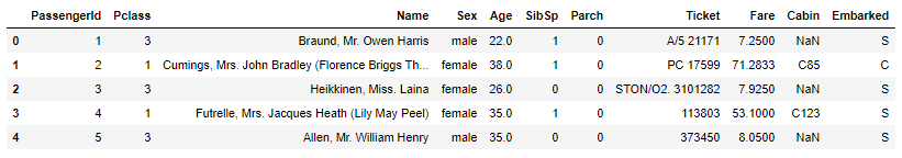
X.head()
# (1309, 11)
3-1. 前処理(全体)
まず、欠損値がどの程度あるのかを確認します。
X.isnull().sum()

'''
PassengerId       0
Pclass            0
Name              0
Sex               0
Age             263
SibSp             0
Parch             0
Ticket            0
Fare              1
Cabin          1014
Embarked          2
dtype: int64
'''
文字列データのままでは、モデルの作成をすることができないため
随時、数値に変換をしていきます。
性別について、「男性:0、女性:1」に変換します。
def code_transform(x):

    if x == 'male':
        y = 0
    else:
        y = 1

    return y

X['Sex'] = X['Sex'].apply(lambda x: code_transform(x))
X.head()

船に乗った港について、「0:C、1:Q、2:S」に変換します。
def code_transform(x):

    if x == 'C':
        y = 0
    elif x == 'Q':
        y = 1
    else:
        y = 2

    return y

X['Embarked'] = X['Embarked'].apply(lambda x: code_transform(x))
X.head()

ここで、数値だけを含む列と、文字だけを含む列について調べます。
numerical_col = [col for col in X.columns if X[col].dtype != 'object']
categorical_col = [col for col in X.columns if X[col].dtype == 'object']

print(numerical_col)
print(categorical_col)

# ['PassengerId', 'Pclass', 'Sex', 'Age', 'SibSp', 'Parch', 'Fare', 'Embarked']
# ['Name', 'Ticket', 'Cabin']
数値カラムと文字列カラムについて、別々の前処理をしたいので分離します。
X_num = X[numerical_col]
X_cat = X[categorical_col]

print(X_num.shape)
print(X_cat.shape)

# (1309, 8)
# (1309, 3)
3-2. 前処理(数値カラム)
データの中身を確認しておきます。
X_num.head()

欠損値をそれぞれの列の中央値で埋めます。
X_num.fillna(X_num.median(), inplace=True)
欠損値の状態を確認します。
X_num.isnull().sum()

'''
PassengerId    0
Pclass         0
Sex            0
Age            0
SibSp          0
Parch          0
Fare           0
Embarked       0
dtype: int64
'''
3-3. 前処理(文字列カラム)
データの中身を確認しておきます。
X_cat.head()

欠損値には、一貫して'missing'の文字を入れます。
X_cat.fillna(value='missing', inplace=True)
欠損値の状態を確認します。
X_cat.isnull().sum()

'''
Name      0
Ticket    0
Cabin     0
dtype: int64
'''
One-Hot-Encodingをして、文字列を全て数値に変換します。
X_cat = pd.get_dummies(X_cat)

print(X_cat.shape)
X_cat.head()

# (1309, 2422)

3-4. 前処理(全体)
X_numとX_catは、両方とも欠損値がなくなり、数値のみのデータとなったので
結合して全体のデータに戻します。
X_total = pd.concat([X_num, X_cat], axis=1)

print(X_total.shape)
X_total.head()

# (1309, 2431)

trainデータのみでモデルを作成したいですが
X_totalはtestデータも含んでしまっているため、必要な部分のみを抽出します。
train_rows = train.shape[0]
X = X_total[:train_rows]

std = StandardScaler()
X = std.fit_transform(X)

print(X.shape)
print(y.shape)

# (891, 2431)
# (891,)
# 4. モデルの作成 trainデータに該当する特徴量と目的変数が揃ったので さらに学習データとテストデータに分けて、モデルの作成をしていきます。
X_train, X_test, y_train, y_test = train_test_split(X, y, test_size=0.3, random_state=123)

print(X_train.shape)
print(y_train.shape)
print(X_test.shape)
print(y_test.shape)

# (623, 2431)
# (623,)
# (268, 2431)
# (268,)
logreg = LogisticRegression(class_weight='balanced')
logreg.fit(X_train, y_train)

'''
LogisticRegression(C=1.0, class_weight='balanced', dual=False,
                   fit_intercept=True, intercept_scaling=1, l1_ratio=None,
                   max_iter=100, multi_class='auto', n_jobs=None, penalty='l2',
                   random_state=None, solver='lbfgs', tol=0.0001, verbose=0,
                   warm_start=False)
'''
次に予測値を求めます。
y_probaに[ : , 1]を指定することで、Class1(Survived=1)になる確率を予測します。
y_predは0.5よりも大きければ1を、小さければ0を振り分けています。
y_proba = logreg.predict_proba(X_test)[: , 1]
print(y_proba[:5])

y_pred = logreg.predict(X_test)
print(y_pred[:5])

# [0.90784721 0.09948558 0.36329043 0.18493678 0.43881127]
# [1 0 0 0 0]
## 5. 性能評価 ROC曲線とAUCを用いて評価します。
fpr, tpr, thresholds = roc_curve(y_test, y_proba)
auc_score = roc_auc_score(y_test, y_proba)
plt.plot(fpr, tpr, label='AUC = %.3f' % (auc_score))
plt.legend()
plt.title('ROC curve')
plt.xlabel('False Positive Rate')
plt.ylabel('True Positive Rate')
plt.grid(True)

print('accuracy:',accuracy_score(y_test, y_pred))
print('f1_score:',f1_score(y_test, y_pred))

# accuracy: 0.7723880597014925
# f1_score: 0.6013071895424837

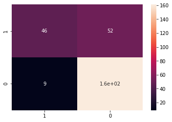
また、混同行列も用いて評価してみます。
classes = [1, 0]
cm = confusion_matrix(y_test, y_pred, labels=classes)

cmdf = pd.DataFrame(cm, index=classes, columns=classes)

sns.heatmap(cmdf, annot=True)
print(classification_report(y_test, y_pred))
'''
              precision    recall  f1-score   support

           0       0.76      0.95      0.84       170
           1       0.84      0.47      0.60        98

    accuracy                           0.77       268
   macro avg       0.80      0.71      0.72       268
weighted avg       0.79      0.77      0.75       268

'''
6. Submit
trainデータを用いて、モデルの作成・評価ができたので
testデータの情報を与えて、予測値を出していきます。
まず全体データ(X_total)のうち、testデータに該当する部分を抽出します。
X_submit = X_total[train_rows:]
X_submit = std.fit_transform(X_submit)

print(X_train.shape)
print(X_submit.shape)

# (623, 2431)
# (418, 2431)
モデルを作成したX_trainと比較して、同じ特徴量数(2431)になっているので
X_submitをモデルに投入して、予測値を出します。
y_proba_submit = logreg.predict_proba(X_submit)[: , 1]
print(y_proba_submit[:5])

y_pred_submit = logreg.predict(X_submit)
print(y_pred_submit[:5])

# [0.02342065 0.18232356 0.06760457 0.06219097 0.76277487]
# [0 0 0 0 1]
KaggleへSubmit(提出)するCSVデータを用意します。
まず、必要な情報を揃えたデータフレームを作成します。
df_submit = pd.DataFrame(y_pred_submit, index=PassengerId, columns=['Survived'])
df_submit.head()

その後、CSVデータに変換します。
df_submit.to_csv('titanic_submit.csv')
これで、Submitをして終了です。

■ 最後に
今回はKaggle初心者の方に向けて、記事をまとめさせていただきました。
少しでもお役に立てたようでしたら幸いです。
ご精読いただきありがとうございました。