はじめに

中心極限定理に代表される確率分布の漸近的性質をPythonで可視化してみました。
漸近的性質は、主に、書籍「日本統計学会公式認定統計検定1級対応統計学」に載っているものを抜粋しました。

中心極限定理

確率分布$X_i(i=1,\cdots,n)$が，平均$\mu$，分散$\sigma^2$の独立同分布に従うとする。$\frac{\sum_{i=1}^nX_i}{n}$は$n\to \infty$のとき、平均$\mu$，分散$ \frac{\sigma^2}{n}$の正規分布に従う。

実験

せっかくなので歪んだ分布で実験を実施する。$X_i(i=1,\cdots,n)$の密度関数を

f(x) = 11 x^{10}\ \ \ (0\leq x\leq1)

とする。

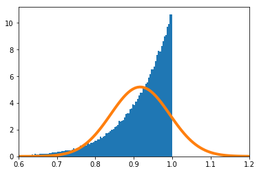
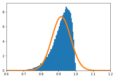
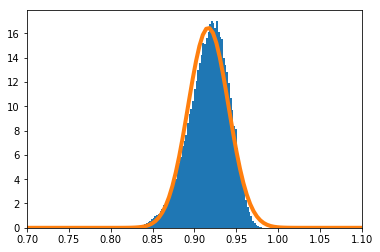
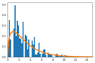
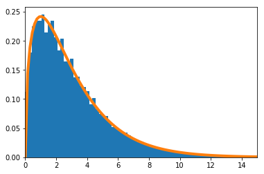
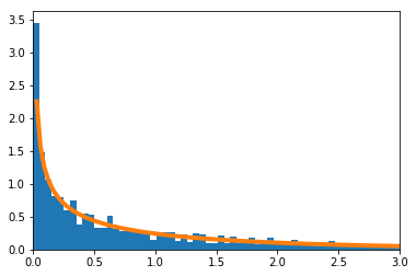
$\frac{\sum_{i=1}^nX_i}{n}$の密度関数を数値的に求めたのが青のヒストグラム、理論上収束するとされる正規分布の密度関数がオレンジの実線である。

$n=1$
$n=2$
$n=10$の場合

$n=1$の場合のPythonソースコードはこちら。

import numpy as np
import matplotlib.pyplot as plt
from scipy.stats import norm

# 確率密度関数 平均11/12, 分散11/13-(11/12)^2
def f(x):
    return 11 * (x ** 10)
mu = 11 / 12
sigma2 = 11 / 13 - (11 / 12) ** 2
# 累積分布関数
def F(x):
    return x ** 11
# 累積分布関数の逆関数
def F_inv(x):
    return x ** (1 / 11)

n = 1
xmin = 0.6
xmax = 1.2
meanX = []
for _ in range(100000):
    meanX.append(np.sum(F_inv(np.random.rand(n))) / n)
plt.hist(meanX, bins=200, density=True)
s = np.linspace(xmin, xmax, 100)
plt.plot(s, norm.pdf(s, mu, (sigma2 / n) ** 0.5), linewidth=4)
plt.xlim(xmin, xmax)

適合度検定の統計検定量（その1）

$(X_1,X_2,\cdots,X_m)$が、試行回数$n$、確率$(p_1,p_2,\cdots,p_m)$の多項分布に従うとする。

\sum_{i=1}^m\frac{(X_i-np_i)^2}{np_i}

は、$n\to \infty$のとき自由度$(m-1)$の$\chi^2$分布に従う。

実験

確率が$\big(\frac{1}{16},\frac{1}{4},\frac{1}{4},\frac{7}{16}\big)$の4項分布で考える。数値的に求めた

\sum_{i=1}^4\frac{(X_i-np_i)^2}{np_i}

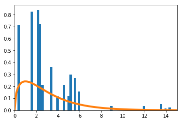
を青のヒストグラムで、理論上収束するとされる自由度3の$\chi^2$分布をオレンジの実線で示す。

$n=4$
$n=16$
$n=400$

$n=4$の場合のPythonソースコードはこちら。

import numpy as np
import matplotlib.pyplot as plt
from scipy.stats import chi2
p = [1/16, 1/4, 1/4, 7/16]
n = 4
xmin = 0
xmax = 15
xx = []
for _ in range(100000):
    r = np.random.rand(1, n)
    x = [0] * 4
    x[0] = np.sum(r < sum(p[:1]))
    x[1] = np.sum(np.logical_and(sum(p[:1]) <= r, r < sum(p[:2])))
    x[2] = np.sum(np.logical_and(sum(p[:2]) <= r, r < sum(p[:3])))
    x[3] = np.sum(sum(p[:3]) <= r)
    xx.append(sum([(x[i] - n * p[i]) ** 2 / (n * p[i]) for i in range(4)]))
plt.hist(xx, bins=int(max(xx))*5, density=True)
s = np.linspace(xmin, xmax, 100)
plt.plot(s, chi2.pdf(s, 3), linewidth=4)
plt.xlim(xmin, xmax)

適合度検定の統計検定量（その2）

真の確率$p_i(i=1,2,\cdots,m)$が未知であるが、$p_i$は$l$次元のパラメータ$\boldsymbol{\theta}(l\leq m-2)$で表現できることが分かっているとする。$p_i$の最尤推定量を$\hat{p}_i$とするとき、

\sum_{i=1}^m\frac{(X_i-n\hat{p}_i)^2}{n\hat{p}_i}

は、$n\to \infty$のとき自由度$(m-l-1)$の$\chi^2$分布に従う。

実験

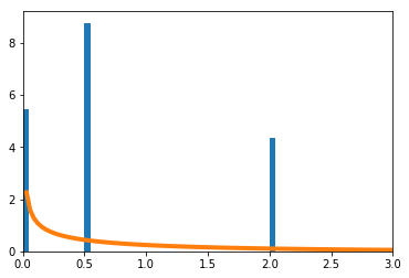
確率が$\big(\frac{1}{16},\frac{1}{4},\frac{1}{4},\frac{7}{16}\big)$の4項分布で考える。真の$p$は未知であるが、$p_2=p_3$だけは既知とする。このとき、$p = [q,r,r,1-2r-q]$と表現できる。$q,r$を最尤推定法で求める。

\sum_{i=1}^m\frac{(X_i-n\hat{p}_i)^2}{n\hat{p}_i}

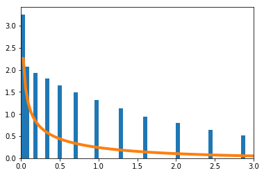
を青のヒストグラムで、理論上収束するとされる自由度1の$\chi^2$分布をオレンジで示す。

$n=4$
$n=100$
$n=10000$

$n=4$の場合のPythonソースコードはこちら。

import numpy as np
import matplotlib.pyplot as plt
from scipy.stats import chi2
n = 4
xmin = 0
xmax = 3
xx = []
for _ in range(100000):
    r = np.random.rand(1, n)
    x = [0] * 4
    x[0] = np.sum(r < sum(p[:1]))
    x[1] = np.sum(np.logical_and(sum(p[:1]) <= r, r < sum(p[:2])))
    x[2] = np.sum(np.logical_and(sum(p[:2]) <= r, r < sum(p[:3])))
    x[3] = np.sum(sum(p[:3]) <= r)
    p_ = [0] * 4
    p_[0] = x[0] / sum(x)
    p_[1] = (x[1] + x[2]) / (2 * sum(x))
    p_[2] = (x[1] + x[2]) / (2 * sum(x))
    p_[3] = x[3] / sum(x)  
    xx.append(sum([(x[i] - n * p_[i]) ** 2 / (n * p[i]) for i in range(4)]))
plt.hist(xx, bins=int(max(xx))*20, density=True)
s = np.linspace(xmin, xmax, 100)
plt.plot(s, chi2.pdf(s, 1), linewidth=4)
plt.xlim(xmin, xmax)

最尤推定量の漸近正規性（その1）

パラメータ$\theta$で特徴づけられた確率変数$X_i(i=1,\cdots,n)$について、$\theta_0$を真のパラメータ、$\hat\theta$を最尤推定量、フィッシャー情報量を$J_n(\theta)$を

J_n(\theta)=E_\theta\Big[\Big(\frac{\delta}{\delta\theta}\log f(X_1,...,X_n;\theta)\Big)^2\Big]

とする。$\hat\theta$は$n\to \infty$のとき平均$\theta_0$、分散$J_n(\theta_0)^{-1}$の正規分布に従う。

実験

$X_i(i=1,\cdots,n)$の密度関数を

f(x) = (\theta+1) x^{\theta}\ \ \ (0\leq x\leq1)

とする。真の$\theta$を10とする。

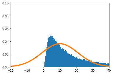
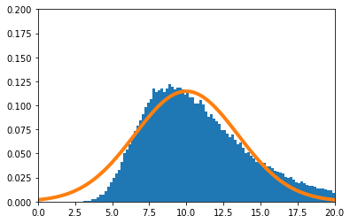
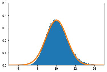
実験的に求めた$\hat\theta$の分布を青のヒストグラム、理論上収束するとされる正規分布をオレンジで示す。

$n=1$
$n=10$
$n=100$

$n=1$のときのPythonソースコードはこちら。

import numpy as np
import matplotlib.pyplot as plt
from scipy.stats import norm
# 確率密度関数 平均11/12, 分散11/13-(11/12)^2
def f(x):
    return 11 * (x ** 10)
mu = 11 / 12
sigma2 = 11 / 13 - (11 / 12) ** 2
# 累積分布関数
def F(x):
    return x ** 11
# 累積分布関数の逆関数
def F_inv(x):
    return x ** (1 / 11)

n = 1
theta_min = -20
theta_max = 40
theta = []
for _ in range(100000):
    x = F_inv(np.random.rand(n))
    theta.append(- n / sum(np.log(x)) - 1)
theta = np.array(theta)

# thetaのヒストグラム
th = np.linspace(theta_min, theta_max, 100)
hi = np.array([np.sum(np.logical_and(th[i] < theta, theta <= th[i + 1])) for i in range(100 - 1)]) / (len(theta) * (th[1] - th[0]))
plt.bar((th[:-1] + th[1:]) / 2, hi, width=(th[1] - th[0]))
# 正規分布
s = np.linspace(theta_min, theta_max, 100)
plt.plot(s, norm.pdf(s, 10, (11 ** 2 / n) ** 0.5), 'tab:orange', linewidth=4)
plt.xlim(theta_min, theta_max)
plt.ylim(0.0, 0.1)

最尤推定量の漸近正規性（その2）

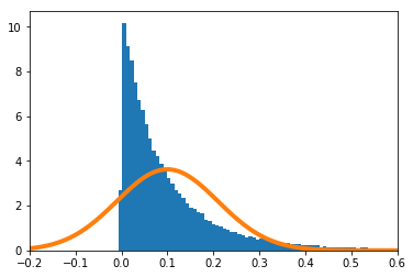
$g$を$\theta_0$で微分可能な関数とする。$g(\hat\theta)$は$n \to \infty$のとき、平均$g(\theta_0)$、分散$g^\prime (\theta_0)^2 J_n(\theta_0)^{-1}$の正規分布に従う。ただし、$\theta$、$\hat\theta$、$\theta_0$の定義は、その1と同じである。

実験

その1の続きの実験をする。$g$を下式で定義する。

g(\theta)=\frac{1}{\theta}

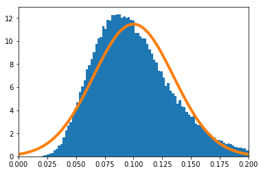
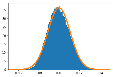
実験的に求めた$g(\hat\theta)$の分布を青のヒストグラム、理論上収束するとされる正規分布をオレンジで示す。

$n=1$
$n=10$
$n=100$

$n=1$の場合のPythonソースコードはこちら。

import numpy as np
import matplotlib.pyplot as plt
from scipy.stats import norm

# 確率密度関数 平均11/12, 分散11/13-(11/12)^2
def f(x):
    return 11 * (x ** 10)
mu = 11 / 12
sigma2 = 11 / 13 - (11 / 12) ** 2
# 累積分布関数
def F(x):
    return x ** 11
# 累積分布関数の逆関数
def F_inv(x):
    return x ** (1 / 11)

n = 1
theta_min = -0.2
theta_max = 0.6
theta = []
for _ in range(100000):
    x = F_inv(np.random.rand(n))
    theta.append(1 / (- n / sum(np.log(x)) - 1))
theta = np.array(theta)
th = np.linspace(theta_min, theta_max, 100)
hi = np.array([np.sum(np.logical_and(th[i] < theta, theta <= th[i + 1])) for i in range(100 - 1)]) / (len(theta) * (th[1] - th[0]))
plt.bar((th[:-1] + th[1:]) / 2, hi, width=(th[1] - th[0]))
s = np.linspace(theta_min, theta_max, 100)
plt.plot(s, norm.pdf(s, 1/10, (11 ** 2 / n / 10 ** 4) ** 0.5), 'tab:orange', linewidth=4)
plt.xlim(theta_min, theta_max)

尤度比検定の統計検定量

パラメータ$\theta$で特徴づけられた確率分布$f(x;\theta)$が存在するとする。仮説検定問題

$H_0:\theta\in\Theta_0$ vs. $H_1:\theta\in\Theta_1 $

において、尤度比$L$は次式で定義される。

L=\frac{\sup_{\theta\in\Theta_1} f(x_1,\cdots,x_n;\theta)}{\sup_{\theta\in\Theta_0} f(x_1,\cdots,x_n;\theta)}

$2\log L$は帰無仮説の下で$n \to \infty$のとき自由度$p$の$\chi^2$分布に従う。ただし、$p＝\dim(\Theta_1) - \dim(\Theta_0)$

実験

f(x;\theta) = (\theta+1) x^{\theta}\ \ \ (0\leq x\leq1)

として、仮説検定問題を

$H_0:\theta=10$ vs. $H_1\neq10 $