More than 3 years have passed since last update.

Spotify API で遊ぶ ~NetworkX で関連アーティストを可視化~

Posted at 2021-09-10

Spotify API で色々な情報を取得できると知り、面白そうだったので遊んでみました。
n 番煎じですが、あるアーティストに対して、その関連アーティストをグラフにして可視化してみます。

今回のプログラムは Google Colab で実行できるようにしています。
https://colab.research.google.com/drive/1Aev5FZ3an13QMwJuJzP9Ahekv_Oosfs1?usp=sharing

GitHub は以下。
https://github.com/yousukeayada/spotify

環境

macOS Catalina 10.15.6
Python 3.8.1
spotipy==2.19.0
networkx==2.6.2

API のテスト

まず Spotify for Developers にログインして create an app
https://developer.spotify.com/dashboard/
作成できたら client id と client secret をメモっておきます。

Python のライブラリ spotipy を使ってテストします。

pip install spotipy

まず、指定したアーティストの情報を取得してみます。
https://spotipy.readthedocs.io/en/2.19.0/#getting-started
アーティスト ID は、アプリだと「リンクをシェア」から URL がわかるので、そこから抜き出します。

import json

import spotipy
from spotipy.oauth2 import SpotifyClientCredentials

def auth_spotify():
    client_id     = "xxxxx"
    client_secret = "xxxxx"

    client_credentials_manager = SpotifyClientCredentials(client_id, client_secret)
    return spotipy.Spotify(client_credentials_manager=client_credentials_manager, language='en')

spotify = auth_spotify()

name_id = {"Sambomaster": "5ydDSP9qSxEOlHWnpbblFB", "FLOW": "3w2HqkKa6upwuXEULtGvnY"}
artist_info = spotify.artist(name_id["Sambomaster"])
print(json.dumps(artist_info))

出力を jq コマンドで整形したものが以下になります。

artist.json

{
  "external_urls": {
    "spotify": "https://open.spotify.com/artist/5ydDSP9qSxEOlHWnpbblFB"
  },
  "followers": {
    "href": null,
    "total": 240331
  },
  "genres": [
    "j-pop",
    "j-poprock",
    "j-rock"
  ],
  "href": "https://api.spotify.com/v1/artists/5ydDSP9qSxEOlHWnpbblFB",
  "id": "5ydDSP9qSxEOlHWnpbblFB",
  "images": [
    {
      "height": 640,
      "url": "https://i.scdn.co/image/ab6761610000e5ebb83514fcda99f392cabbb051",
      "width": 640
    },
    {
      "height": 320,
      "url": "https://i.scdn.co/image/ab67616100005174b83514fcda99f392cabbb051",
      "width": 320
    },
    {
      "height": 160,
      "url": "https://i.scdn.co/image/ab6761610000f178b83514fcda99f392cabbb051",
      "width": 160
    }
  ],
  "name": "Sambomaster",
  "popularity": 53,
  "type": "artist",
  "uri": "spotify:artist:5ydDSP9qSxEOlHWnpbblFB"
}

次に、関連アーティストの取得です。

# （略）

artist_info = spotify.artist(name_id["Sambomaster"])
artist_id = artist_info["id"]

related_artists = spotify.artist_related_artists(artist_id)
print(json.dumps(related_artists))

出力（長いので一部のみ）

related_artists.json

{
  "artists": [
    {
      "external_urls": {
        "spotify": "https://open.spotify.com/artist/2dP0aHVXt8dDPCw5d2Jw0m"
      },
      "followers": {
        "href": null,
        "total": 138679
      },
      "genres": [
        "j-pop",
        "j-poprock",
        "j-rock",
        "japanese alternative rock",
        "japanese punk rock"
      ],
      "href": "https://api.spotify.com/v1/artists/2dP0aHVXt8dDPCw5d2Jw0m",
      "id": "2dP0aHVXt8dDPCw5d2Jw0m",
      "images": [
        {
          "height": 640,
          "url": "https://i.scdn.co/image/ab6761610000e5eb2b458dd9eb80278b2566d299",
          "width": 640
        },
        {
          "height": 320,
          "url": "https://i.scdn.co/image/ab676161000051742b458dd9eb80278b2566d299",
          "width": 320
        },
        {
          "height": 160,
          "url": "https://i.scdn.co/image/ab6761610000f1782b458dd9eb80278b2566d299",
          "width": 160
        }
      ],
      "name": "GING NANG BOYZ",
      "popularity": 47,
      "type": "artist",
      "uri": "spotify:artist:2dP0aHVXt8dDPCw5d2Jw0m"
    },
    {
      "external_urls": {
    ...
}

以上でテスト完了です。

NetworkX で可視化

Google Colab を使う場合は元から入っています。

pip install networkx

有向グラフで可視化します。単にグラフを描画するだけだと複雑で見辛いので、ここではいくつかルールを設けます。

popularity が大きいほどノードを大きくする
in_degree （自分に向かう矢印）が多いほどノードの色を濃くする

グラフを見やすくする工夫は他にもたくさんあると思います。例えば、ジャンルに j-rock が含まれているものだけ色を変えるなど、目的に応じて設定すればいいでしょう。

from ast import literal_eval

import pandas as pd
import networkx as nx
import matplotlib.pyplot as plt
from matplotlib.font_manager import FontProperties


artists_df = pd.read_csv("artists.csv", converters={"genres":literal_eval, "related_artist_ids":literal_eval, "related_artist_names":literal_eval})

G = nx.MultiDiGraph()

# node データの追加
names = [name for name in artists_df["name"]]
G.add_nodes_from(names)

edges = []
for name, related_artist_names in zip(artists_df["name"], artists_df["related_artist_names"]):
    for related_name in related_artist_names:
        if related_name in names:
            e = (name, related_name)
            edges.append(e)
            # print(e)

# edge データの追加
G.add_edges_from(edges)

for d in zip(*G.in_degree()):
    max_in_degree = max(d)

plt.figure(figsize=(30, 30), dpi=300)
pos = nx.spring_layout(G, k=0.3, seed=23)

node_size = [popularity*40 for popularity in artists_df["popularity"]]
# in_degree を正規化して alpha とする
node_alpha = [d[1] / max_in_degree for d in G.in_degree()]
nx.draw_networkx_nodes(G, pos, node_color='red',alpha=node_alpha, node_size=node_size, edgecolors="black")
text_items = nx.draw_networkx_labels(G, pos, font_size=5, font_weight="bold")
nx.draw_networkx_edges(G, pos, alpha=0.4, edge_color='royalblue')

# 日本語フォントを使う
font_prop = FontProperties(fname="/System/Library/Fonts/ヒラギノ角ゴシック W8.ttc", weight=1000, size=5)
for t in text_items.values():
    t.set_fontproperties(font_prop)

plt.savefig("network.png")

これで可視化した画像が保存されます。

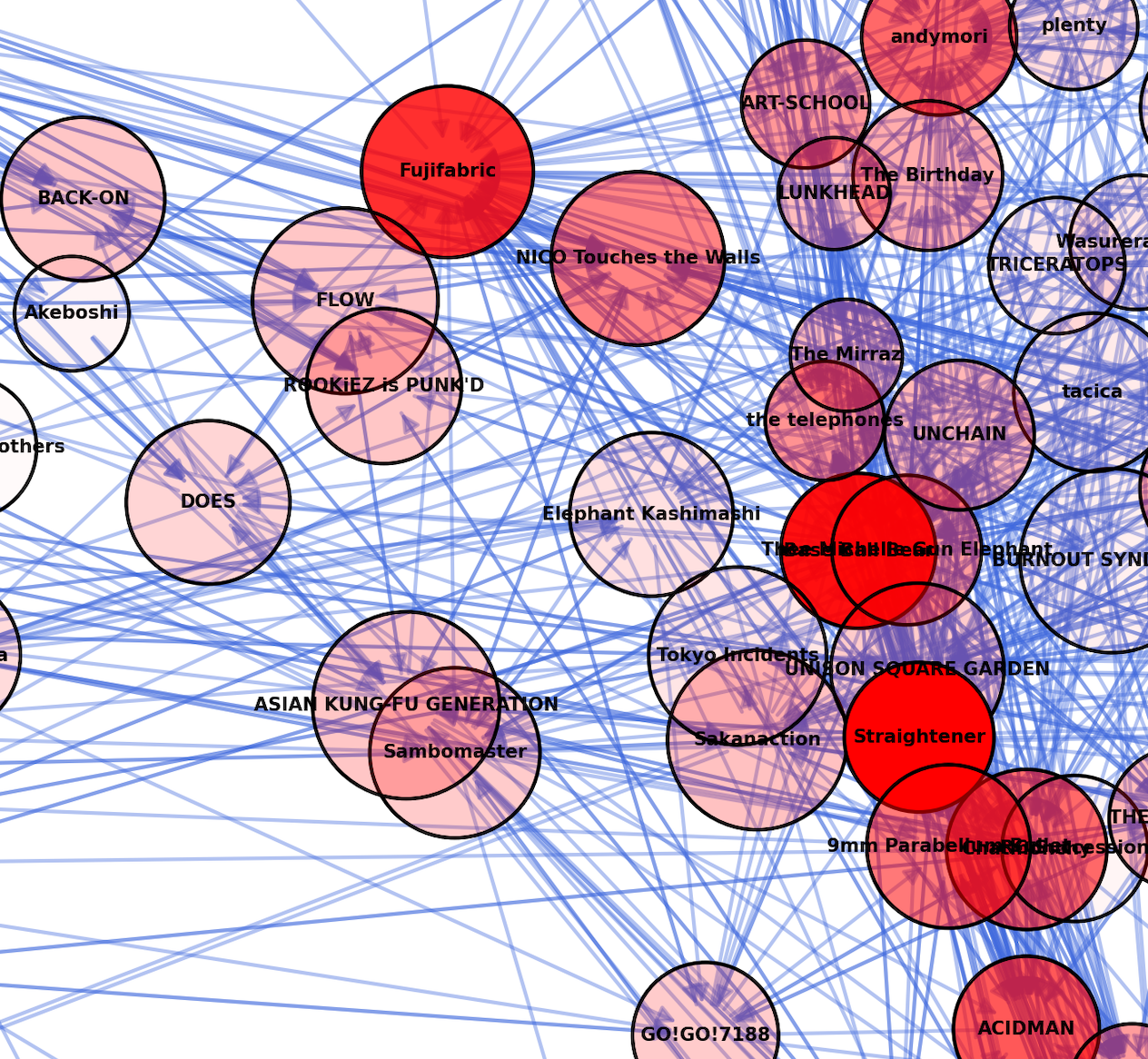
サンボマスターを起点とした場合、以下のようなグラフとなりました。

なんとなく 2 つグループに分かれていることが読み取れますが、詳しくはわからないので、拡大して見てみましょう。
真ん中左あたりにコブクロ、いきものがかり、スキマスイッチなど、テレビでもよく見るようなアーティストが集まっていることがわかります。

in_degree が最も多かったのは Straightener 、次点で Base Ball Bear でした。

別のアーティストでもやってみます。

FLOW を指定してみるとわかりやすく複数のグループにわかれました。詳細は画像参照。

また、それぞれのグループの間に橋渡し的な存在を確認できます。例えば、青色と紫色を繋ぐのは UVERworld 、青とオレンジを繋ぐのは藍井エイル、青と緑は ORANGE RANGE です。

最後に、最近話題の YOASOBI でやってみます。

やはり若者に人気のアーティストが多い感じがします。左下には上記と同じような J-Pop 島があります。 J-Pop はあらゆるジャンルからの導線がありそうですね。

ジャンルの集計

関連アーティストのジャンルを多い順に集計します。

from ast import literal_eval
from collections import defaultdict

import pandas as pd


def count_genres(artists_df):
    genres_dict = defaultdict(int)
    for genres in artists_df["genres"]:
        for g in genres:
            genres_dict[g] += 1
    genres_dict = sorted(genres_dict.items(), key=lambda x:x[1], reverse=True)

    genres_dict2 = {}
    for k, v in genres_dict:
        genres_dict2[k] = v
    return genres_dict2

artists_df = pd.read_csv("artists.csv", converters={"genres":literal_eval, "related_artist_ids":literal_eval, "related_artist_names":literal_eval})

genres_dict = count_genres(artists_df)
for k, v in genres_dict.items():
    print(k, v)

先ほどの YOASOBI だと以下のような結果が得られます。

j-pop 117
j-rock 53
j-poprock 42
anime 29
japanese alternative rock 24
japanese teen pop 23
anime rock 16
vocaloid 10
japanese r&b 9
japanese singer-songwriter 8
j-division 6
j-pop boy group 6
j-acoustic 5
japanese indie rock 5
japanese soul 4
j-pixie 4
japanese pop rap 4
j-idol 4
japanese electropop 3
j-rap 3
classic j-pop 3
j-pop girl group 3
j-indie 3
japanese punk rock 2
japanese emo 2
japanese alternative pop 1
japanese new wave 1
city pop 1
japanese trap 1
kyushu indie 1
kawaii edm 1
japanese vtuber 1
honeyworks 1
j-punk 1
japanese pop punk 1
visual kei 1
japanese shoegaze 1
hokkaido indie 1
okinawan folk 1
okinawan pop 1
japanese indie pop 1

枝刈り

エッジが多すぎて見辛い場合は枝刈りをするといいでしょう。試しに単方向のエッジを削除して、双方向のみ残します。

import networkx as nx

def remove_unidirectional(G):
    unidirectional = [(u, v) for u, v in G.edges() if not (v, u) in G.edges()]
    for u, v in unidirectional:
        G.remove_edge(u, v)
    return G

G = nx.MultiDiGraph()
# （中略）
print(G.number_of_edges()) # 枝刈り前
G = remove_unidirectional(G)
print(G.number_of_edges()) # 枝刈り後

# 以下グラフ描画
# ...