回帰分析については以前にも線形回帰の話題で触れました。
NumPy で回帰分析
では実際にコードを書いて回帰分析をおこなってみます。 np.polyfit や np.polyval を利用すると n 次式で 2 変数の回帰分析をおこなえます。
詳細は上記のリンクからドキュメントを参照したほうが良いのですが、次の通りとなります。
- np.polyfit(x, y, n) : n 次式で 2 変数の回帰分析
- np.polyval(p, t) : p で表される多項式に t を代入し値を計算
import numpy as np
import matplotlib.pyplot as plt
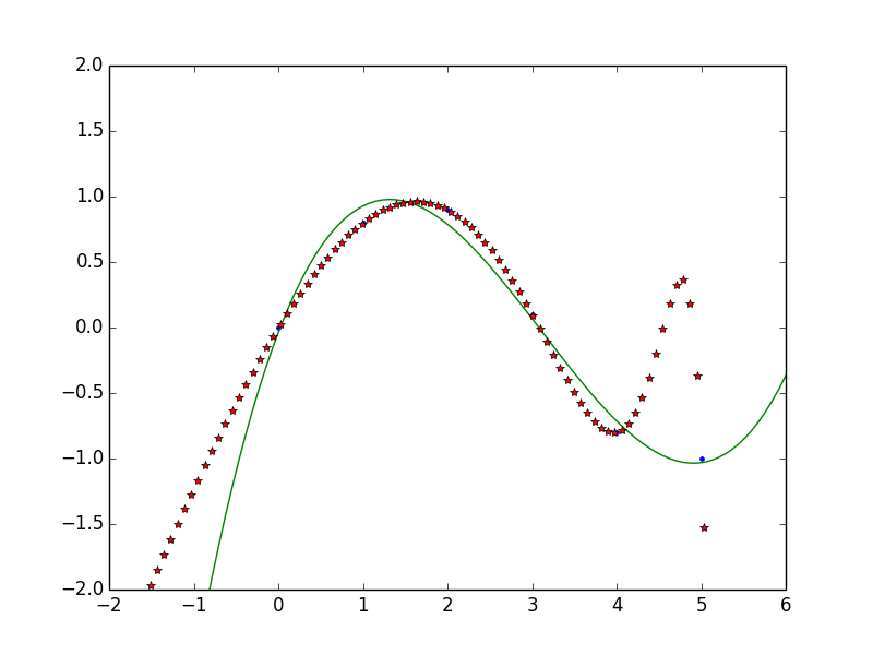
x = np.array([0.0, 1.0, 2.0, 3.0, 4.0, 5.0])
y = np.array([0.0, 0.8, 0.9, 0.1, -0.8, -1.0])
z = np.polyfit(x, y, 3)
p = np.poly1d(z)
p30 = np.poly1d(np.polyfit(x, y, 30))
xp = np.linspace(-2, 6, 100)
plt.plot(x, y, '.', xp, p(xp), '-', xp, p30(xp), '*')
plt.ylim(-2,2)
plt.show()
plt.savefig('image.png')
このとき
1 次式の場合は p[0]: 傾き、 p[1]: 切片となります。
N 次式なら p[0]t*(N-1) + p[1]t*(N-2) + ... + p[N-2]*t + p[N-1] です。
最小二乗法についても以前に触れましたが、データ列 {(x_1, y_1), (x_2, y_2), ... (x_n, y_n)} に対して残差平方和を最小とするモデルを決定します。このとき観測値の誤差分布の分散が一定であると仮定します。
重回帰分析
独立変数 m 個のモデルでの回帰分析が重回帰分析です。
z = ax + by + c
という式を求めたいとします。
x = [9.83, -9.97, -3.91, -3.94, -13.67, -14.04, 4.81, 7.65, 5.50, -3.34]
y = [-5.50, -13.53, -1.23, 6.07, 1.94, 2.79, -5.43, 15.57, 7.26, 1.34]
z = [635.99, 163.78, 86.94, 245.35, 1132.88, 1239.55, 214.01, 67.94, -1.48, 104.18]

import numpy as np
from scipy import linalg as LA

N = len(x)
G = np.array([x, y, np.ones(N)]).T
result = LA.solve(G.T.dot(G), G.T.dot(z))

print(result)
これにより
[ -30.02043308 3.55275314 322.33397214]
が求まりますから
z = -30.0x + 3.55y + 322
という方程式が求まり、これが解となります。
参考
2013年 プログラマの為の数学勉強会 資料
http://nineties.github.io/math-seminar/