【Kaggle】自動車保険の2項分類コンペに挑戦

0. 目次

1. 今回の分析の概要
2. 実装
3. 考察・残された課題

1. 今回の分析の概要

　前記事にて、無事にAidemy データ分析講座を修了することができました。データ分析について、より理解を深めるべく、kaggleのコンペに挑戦しました。

1-1. 開発環境

• Mac M2
• Jupyter notebook

1-2. 使用データ

　kaggleの「Binary Classification of Insurance Cross Selling」というコンペに参加しました。

1-3. 目的

• kaggleのコンペに挑戦する
• 予測精度を上げるための様々な方法を模索する
  　　
  以下から、全体の流れ・具体的なコードを説明します。

2. 実装

Step1: 使用するライブラリのインポート

import pandas as pd
import numpy as np
import matplotlib.pyplot as plt
import seaborn as sns
from sklearn.model_selection import train_test_split
from sklearn.model_selection import KFold
from sklearn.metrics import accuracy_score
import random
import os
from sklearn.preprocessing import StandardScaler
from sklearn.linear_model import LogisticRegression
from sklearn.svm import LinearSVC
from sklearn.ensemble import RandomForestClassifier
import lightgbm as lgb
import xgboost as xgb
import tensorflow as tf

Step2: データの可視化

　まずは、train_data（df）とtest_data（df_test; 提出用）の特徴量を確認していきます。

df['Test_Flag'] = 0
df_test['Test_Flag'] = 1
all_df = pd.concat([df, df_test], axis=0).reset_index(drop=True)

# カテゴリー変数に変換
categorical_list = ['id', 'Driving_License', 'Region_Code', 'Previously_Insured', 'Policy_Sales_Channel', 'Response', 'Test_Flag']

for categorical in categorical_list:
    all_df[categorical] = all_df[categorical].astype('category')    

# train_data/test_data間のデータの偏りを確認
fig, axes = plt.subplots(figsize=(12,8), nrows=2, ncols=3)
binary_col_list = ['Gender', 'Driving_License', 'Previously_Insured', 'Vehicle_Age', 'Vehicle_Damage', 'Response']

for ax, col in zip(axes.flatten(),binary_col_list):
    sns.countplot(x=col, data=all_df, hue='Test_Flag', ax=ax)

上記のグラフより、train_dataとtest_data間のデータの偏りはあまりないことがわかりました。

# ヒストグラムを使って、Age、Annual_Premium、Vintageの分布を表示
fig = sns.FacetGrid(df, col='Response', hue='Response', height=4)
fig.map(sns.histplot, 'Age', bins=30, kde=False)

fig = sns.FacetGrid(df, col='Response', hue='Response', height=4)
fig.map(sns.histplot, 'Annual_Premium', bins=30, kde=False)

fig = sns.FacetGrid(df, col='Response', hue='Response', height=4)
fig.map(sns.histplot, 'Vintage', bins=30, kde=False)

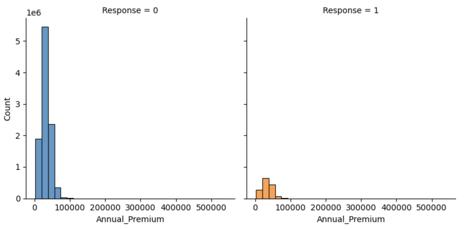
　上記より、以下のことが読み取れました。

• Age: 20代のレスポンス率が低い
• Annual_Premium: 約50000以下だとレスポンス率が低い。分布に偏りがある
• Vintage: 0〜70くらいまでレスポンス率が高い

Step3: データの前処理

(1) 欠損値の処理
　今回のデータに欠損値はなかったので、処理は行いませんでした。

all_df.isnull().sum()

# >>> 出力結果
id                            0
Gender                        0
Age                           0
Driving_License               0
Region_Code                   0
Previously_Insured            0
Vehicle_Age                   0
Vehicle_Damage                0
Annual_Premium                0
Policy_Sales_Channel          0
Vintage                       0
Response                7669866
Test_Flag                     0
# ※Responseの欠損値はtest_dataの分のみでした

(2) 特徴量の追加
　Step2にて、Annual_Premiumの分布に大きく偏りがあること、また、Ageは20代、Vintageは0-70に、レスポンス率の差があることが分かったので、これらのカテゴリ化を行いました。

age_bins =[20, 30, 40, 50, 60, 70, 80, 90]
age_labels=['20s', '30s', '40s','50s', '60s', '70s', '80s']

all_df['AgeBand']=pd.cut(all_df.Age, bins=age_bins, labels=age_labels, right=False)
all_df['AnnualPremiumBand'] = pd.qcut(all_df['Annual_Premium'], 5)
all_df['VintageBand'] = pd.qcut(all_df['Vintage'], 4)

Step4: モデルの比較

　分析を行うに当たり、さまざまなモデルを用いて比較していきます。より正確な評価を行うためにKFold法を使いたかったのですが、データ量が多かったので断念しました。

# シード値の設定
np.random.seed(0)
tf.random.set_seed(0)
random.seed(0)
os.environ['PYTHONHASHSEED'] = str(0)

# カテゴリー変数をOne-Hot Encodingで変換
all_df_base = pd.get_dummies(all_df, columns=['Gender', 'Driving_License', 'Previously_Insured', 'Vehicle_Damage', 'Vehicle_Age', 'AgeBand', 'AnnualPremiumBand', 'VintageBand'])

train_df = all_df_base[all_df_base['Test_Flag']==0]
test_df = all_df_base[all_df_base['Test_Flag']==1]
target = train_df['Response']

# 学習に用いないカラムを削除
drop_col = ['id', 'Region_Code', 'Test_Flag', 'Response', 'Age', 'Annual_Premium', 'Vintage']

train_df = train_df.drop(columns=drop_col)
test_df = test_df.drop(columns=drop_col)

# データ量が大きいため、データを標準化
scaler = StandardScaler()
train_df_scaled = scaler.fit_transform(train_df)
test_df_scaled = scaler.transform(test_df)

train_df_scaled = pd.DataFrame(train_df_scaled, columns=train_df.columns)
test_df_scaled = pd.DataFrame(test_df_scaled, columns=test_df.columns)

# モデルを比較する関数を定義
def comparison(model, X, y):
    X_train, X_val, y_train, y_val = train_test_split(X, y, random_state=0, shuffle=True)

    model.fit(X_train, y_train)
    print(f'train_dataのスコアは{accuracy_score(y_train, model.predict(X_train))}, val_dataのスコアは{accuracy_score(y_val, model.predict(X_val))}')

# MLPモデルを比較する関数を定義
def comparison_mlp():
    target_mlp = target.astype('float64')
    X_train, X_val, y_train, y_val = train_test_split(train_df_scaled, target_mlp, random_state=0, shuffle=True)
    
    model_mlp = tf.keras.models.Sequential([
            tf.keras.layers.Input((X_train.shape[1],)),
            tf.keras.layers.Dense(32, activation='relu'),
            tf.keras.layers.Dropout(0.5),
            tf.keras.layers.Dense(16, activation='sigmoid'),
            tf.keras.layers.Dense(1,activation='sigmoid')
        ])
    model_mlp.compile(optimizer='adam', loss='binary_crossentropy', metrics=['accuracy'])
    early_stopping = tf.keras.callbacks.EarlyStopping(monitor='val_loss', patience=10, restore_best_weights=True)
    model_mlp.fit(X_train, y_train, epochs=100, verbose=0, batch_size=32, callbacks=[early_stopping])

    y_train_pred = (model_mlp.predict(X_train) > 0.5).astype(int)
    y_val_pred = (model_mlp.predict(X_val) > 0.5).astype(int)
    
    print(f'train_dataのスコアは{accuracy_score(y_train, y_train_pred)}, val_dataのスコアは{accuracy_score(y_val, y_val_pred)}')

　実際に、モデル同士を比較していきます。

クリックで折りたたみ

# Logistic Regression
model_LR = LogisticRegression()
comparison(model_LR, train_df_scaled, target)

# >>> 出力結果
train_dataのスコアは0.8769917198599355, val_dataのスコアは0.8769146790904666

# SVM
model_svm = LinearSVC(random_state=0)
comparison(model_svm, train_df_scaled, target)

# >>> 出力結果
train_dataのスコアは0.877020345599598, val_dataのスコアは0.8769497948682289

# RandomForest
model_RF = RandomForestClassifier(n_estimators=50, random_state=0, n_jobs=-1)
comparison(model_RF, train_df_scaled, target)

# >>> 出力結果
train_dataのスコアは0.8777701777275984, val_dataのスコアは0.876757527292956

# LightGBM
rename_dict = {'AnnualPremiumBand_(2629.999, 23158.0]':'AnnualPremiumBand_1',
              'AnnualPremiumBand_(23158.0, 29342.0]':'AnnualPremiumBand_2',
              'AnnualPremiumBand_(29342.0, 34794.0]':'AnnualPremiumBand_3',
              'AnnualPremiumBand_(34794.0, 43169.0]':'AnnualPremiumBand_4',
              'AnnualPremiumBand_(43169.0, 540165.0]':'AnnualPremiumBand_5',
              'VintageBand_(9.999, 99.0]':'VintageBand_1',
              'VintageBand_(99.0, 166.0]':'VintageBand_2',
              'VintageBand_(166.0, 232.0]':'VintageBand_3',
              'VintageBand_(232.0, 299.0]':'VintageBand_4'}

train_df_scaled_lgb = train_df_scaled.rename(columns=rename_dict)
model_lgb = lgb.LGBMClassifier(boosting_type='gbdt', objective='binary', metric='binary_error', seed=0, verbose=0, n_jobs=-1)
comparison(model_lgb, train_df_scaled_lgb, target)

# >>> 出力結果
train_dataのスコアは0.8771883914397217, val_dataのスコアは0.8771778735832001

# XGBoost
rename_dict = {'AnnualPremiumBand_(2629.999, 23158.0]':'AnnualPremiumBand_1',
              'AnnualPremiumBand_(23158.0, 29342.0]':'AnnualPremiumBand_2',
              'AnnualPremiumBand_(29342.0, 34794.0]':'AnnualPremiumBand_3',
              'AnnualPremiumBand_(34794.0, 43169.0]':'AnnualPremiumBand_4',
              'AnnualPremiumBand_(43169.0, 540165.0]':'AnnualPremiumBand_5',
              'VintageBand_(9.999, 99.0]':'VintageBand_1',
              'VintageBand_(99.0, 166.0]':'VintageBand_2',
              'VintageBand_(166.0, 232.0]':'VintageBand_3',
              'VintageBand_(232.0, 299.0]':'VintageBand_4',
              'Vehicle_Age_< 1 Year':'Vehicle_Age_lessthan_1Year',
              'Vehicle_Age_> 2 Years':'Vehicle_Age_morethan_2Year'}

train_df_scaled_xgb = train_df_scaled.rename(columns=rename_dict)
model_xgb = xgb.XGBClassifier(objective='binary:logistic', seed=0, n_estimators=100, max_depth=3, n_jobs=-1)
comparison(model_xgb, train_df_scaled_xgb, target)

# >>> 出力結果
train_dataのスコアは0.8771481763317749, val_dataのスコアは0.8771298936096238

# MLP
comparison_mlp()

# >>> 出力結果
train_dataのスコアは0.877020345599598, val_dataのスコアは0.8769497948682289

　結果は、LightGBMの精度が最も高くなりました。

Step5: モデルの定義・トレーニング・予測

　上記のモデルを使って、モデリングをしていきます。

# 提出用データの作成
rename_dict = {'AnnualPremiumBand_(2629.999, 23158.0]':'AnnualPremiumBand1',
             'AnnualPremiumBand_(23158.0, 29342.0]':'AnnualPremiumBand2',
             'AnnualPremiumBand_(29342.0, 34794.0]':'AnnualPremiumBand_3',
             'AnnualPremiumBand_(34794.0, 43169.0]':'AnnualPremiumBand_4',
             'AnnualPremiumBand_(43169.0, 540165.0]':'AnnualPremiumBand_5',
             'VintageBand_(9.999, 99.0]':'VintageBand_1',
             'VintageBand_(99.0, 166.0]':'VintageBand_2',
             'VintageBand_(166.0, 232.0]':'VintageBand_3',
             'VintageBand_(232.0, 299.0]':'VintageBand_4'}

test_df_scaled_lgb = test_df_scaled.rename(columns=rename_dict)
test_pred_proba = model_lgb.predict_proba(test_df_scaled_lgb)

sample_sub['Response'] = test_pred_proba[:,1]
sample_sub.to_csv("submission.csv", index=False)

　kaggleに提出したところ、スコアは0.86005となり、886位/1412位でした。
（2024/7/19時点)

4. 考察・残された課題

　今回は初めて自力でkaggleのコンペに挑戦してみました。結果は微妙なところでしたが、学びや反省点がいくつか見つかったので、今後も引き続きチャレンジしていきたいと思います。

　 今回のデータセットは量が膨大で、一つ一つの処理にとても時間がかかりました。パラメータの調整や特徴量の追加など試してみたいことはあったのですが、手持ちのパソコンの能力に限界を感じました…しかし、その中でもLightGBMは処理速度が圧倒的に早く、また、精度も高く、強力なアルゴリズムとして広く使われている理由を実感しました。

　 前回のAidemy成果物で作成した世界の幸福度予測モデルでは、データ数が少ないためにLightGBMやXGBoostの精度があまり上がりませんでしたが、今回は最もスコアが良かったのはLightGBMであり、データセットの特性によって最適なモデルが異なるということを改めて学ぶことができました。

　最後まで目を通してくださり、ありがとうございました。