TES インピーダンスの式は見た目が違うだけで実は同じ : Irwin & Hilton と Lindeman et al. 2004 も同じ

はじめに

TES の複素インピーダンスを勉強していると、文献ごとに少しずつ違う式が出てくる。

たとえば、ある導出では TES 単体のインピーダンスを

Z_{\mathrm{TES}}(\omega)
=
R_0(1+\beta)
+
\frac{
R_0(2+\beta)\mathcal{L}
}{
1-\mathcal{L}+i\omega\tau_0
}

と書く。

一方、Irwin & Hilton では、

Z_{\mathrm{TES}}(\omega)
=
R_0(1+\beta_I)
+
\frac{
R_0\mathcal{L}_I
}{
1-\mathcal{L}_I
}
\frac{
2+\beta_I
}{
1+i\omega\tau_I
}

のように書かれる。

さらに Lindeman et al. 2004 では、$\tau_{\mathrm{eff}}$ を使って、また少し違う形で書かれる。

初めて見ると、

式が違う？
符号が違う？
時定数の定義が違う？
どれが正しい？

と混乱しやすい。

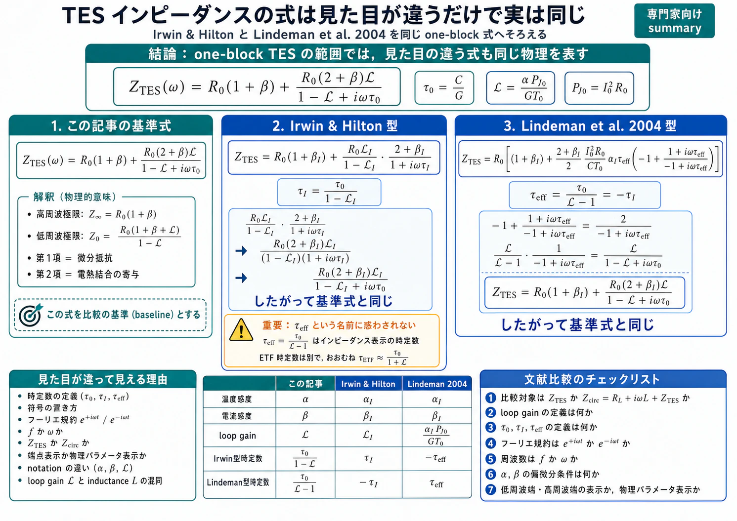
しかし結論から言うと、one-block TES モデルの範囲では、これらは基本的に同じ式である。

違って見える主な理由は、

1. 時定数の定義が違う
2. loop gain の記号が違う
3. フーリエ変換の符号規約が違う
4. TES 単体か、回路全体かが違う
5. f で書くか ω で書くかが違う
6. 低周波端・高周波端で書くか、物理パラメータで直接書くかが違う

というだけである。

この記事では、自分の記事で使う基準式を出発点にして、Irwin & Hilton と Lindeman et al. 2004 の式がどのように同じ形へ変形できるかを整理する。

自分の記事の定義と解説はこちらに書いてます。

この記事の要約

---

1. この記事で使う基準式

この記事では、one-block TES 単体の小信号インピーダンスを次の形で書く。

\boxed{
Z_{\mathrm{TES}}(\omega)
=
R_0(1+\beta)
+
\frac{
R_0(2+\beta)\mathcal{L}
}{
1-\mathcal{L}+i\omega\tau_0
}
}

ここで、

\tau_0=\frac{C}{G}

は自然熱時定数である。

また、

\mathcal{L}
=
\frac{\alpha P_{J0}}{GT_0}

は loop gain である。

平衡点での Joule power は

P_{J0}=I_0^2R_0

である。

$\alpha$ と $\beta$ は、

\alpha
=
\frac{T_0}{R_0}
\left(
\frac{\partial R}{\partial T}
\right)_{I,0}

\beta
=
\frac{I_0}{R_0}
\left(
\frac{\partial R}{\partial I}
\right)_{T,0}

である。

この式を、この記事では「基準式」と呼ぶ。

回路全体のインピーダンスは、TES 単体に直列抵抗と直列インダクタンスを足して、

Z_{\mathrm{circ}}(\omega)
=
R_L+i\omega L+Z_{\mathrm{TES}}(\omega)

である。

この記事で比較したい中心は、基本的には回路全体 $Z_{\mathrm{circ}}$ ではなく、TES 単体の $Z_{\mathrm{TES}}$ である。

---

2. 基準式の物理的な意味

基準式は、

Z_{\mathrm{TES}}(\omega)
=
R_0(1+\beta)
+
\frac{
R_0(2+\beta)\mathcal{L}
}{
1-\mathcal{L}+i\omega\tau_0
}

である。

第一項

R_0(1+\beta)

は、高周波極限の微分抵抗である。

高周波では TES 温度が電流変動に追随できないため、熱応答による第 2 項は消える。したがって、

Z_{\mathrm{TES}}(\infty)
=
R_0(1+\beta)

である。

第二項

\frac{
R_0(2+\beta)\mathcal{L}
}{
1-\mathcal{L}+i\omega\tau_0
}

は、電流変動が Joule heating を変え、それが温度を変え、さらに抵抗を変える、という電熱結合の寄与である。

低周波極限では、

Z_{\mathrm{TES}}(0)
=
R_0(1+\beta)
+
\frac{
R_0(2+\beta)\mathcal{L}
}{
1-\mathcal{L}
}

である。

整理すると、

Z_{\mathrm{TES}}(0)
=
R_0
\frac{
1+\beta+\mathcal{L}
}{
1-\mathcal{L}
}

となる。

$\mathcal{L}>1$ では、低周波側で負の動的抵抗が現れる。これは異常ではなく、電圧バイアス TES の強い electrothermal feedback の反映である。

---

3. Irwin & Hilton の式

Irwin & Hilton では、回路全体の複素インピーダンスを

Z_\omega
=
\frac{V_\omega}{I_\omega}
=
R_L+i\omega L+Z_{\mathrm{TES}}

と書く。

そして、TES 単体の複素インピーダンスを

Z_{\mathrm{TES}}
=
R_0(1+\beta_I)
+
\frac{
R_0\mathcal{L}_I
}{
1-\mathcal{L}_I
}
\frac{
2+\beta_I
}{
1+i\omega\tau_I
}

と書いている。

ここで重要なのは、$\tau_I$ の定義である。

Irwin & Hilton の $\tau_I$ は、

\tau_I
=
\frac{\tau_0}{1-\mathcal{L}_I}

である。

ここで、

\tau_0=\frac{C}{G}

である。

この $\tau_I$ は、いわゆる理想電圧バイアス下の ETF 時定数

\tau_{\mathrm{ETF}}
\simeq
\frac{\tau_0}{1+\mathcal{L}}

とは違う。(ここが最初の重要ポイントである。)

---

4. Irwin & Hilton の式を基準式に直す

Irwin & Hilton の第 2 項だけを見る。

\frac{
R_0\mathcal{L}_I
}{
1-\mathcal{L}_I
}
\frac{
2+\beta_I
}{
1+i\omega\tau_I
}

これを一つの分数にまとめると、

\frac{
R_0\mathcal{L}_I(2+\beta_I)
}{
(1-\mathcal{L}_I)(1+i\omega\tau_I)
}

である。

ここに

\tau_I
=
\frac{\tau_0}{1-\mathcal{L}_I}

を代入する。

分母は、

(1-\mathcal{L}_I)(1+i\omega\tau_I)

である。

これを展開すると、

(1-\mathcal{L}_I)(1+i\omega\tau_I)
=
(1-\mathcal{L}_I)
+
i\omega(1-\mathcal{L}_I)\tau_I

である。

$\tau_I=\tau_0/(1-\mathcal{L}_I)$ なので、

(1-\mathcal{L}_I)\tau_I
=
\tau_0

となる。

したがって、

(1-\mathcal{L}_I)(1+i\omega\tau_I)
=
1-\mathcal{L}_I+i\omega\tau_0

である。

よって、

\frac{
R_0\mathcal{L}_I
}{
1-\mathcal{L}_I
}
\frac{
2+\beta_I
}{
1+i\omega\tau_I
}
=
\frac{
R_0\mathcal{L}_I(2+\beta_I)
}{
1-\mathcal{L}_I+i\omega\tau_0
}

である。

したがって、Irwin & Hilton の式は、

Z_{\mathrm{TES}}
=
R_0(1+\beta_I)
+
\frac{
R_0(2+\beta_I)\mathcal{L}_I
}{
1-\mathcal{L}_I+i\omega\tau_0
}

となる。

これは、この記事の基準式

Z_{\mathrm{TES}}
=
R_0(1+\beta)
+
\frac{
R_0(2+\beta)\mathcal{L}
}{
1-\mathcal{L}+i\omega\tau_0
}

と同じである。

つまり、

\beta_I\leftrightarrow\beta,
\qquad
\mathcal{L}_I\leftrightarrow\mathcal{L}

と読めばよい。

---

5. Irwin & Hilton 式が違って見える理由

Irwin & Hilton の式が違って見える主な理由は、

\tau_I
=
\frac{\tau_0}{1-\mathcal{L}}

を使っているからである。

つまり、自然熱時定数 $\tau_0=C/G$ を明示する代わりに、

\tau_I

という別の時定数で書いている。

そのため、

\frac{1}{1-\mathcal{L}}
\frac{1}{1+i\omega\tau_I}

のように見える。

しかし、分母を一つにまとめれば、

1-\mathcal{L}+i\omega\tau_0

になり、基準式と同じになる。

したがって、Irwin & Hilton の式は、

見た目は違うが、時定数の定義を戻せば同じ

である。

---

6. Lindeman et al. 2004 の式

Lindeman et al. 2004 では、TES 抵抗を小信号で

R
=
R_0
\left(
1+\alpha_I\frac{T}{T_0}
+\beta_I\frac{I}{I_0}
\right)

のように線形化する。

ここで $\alpha_I$ と $\beta_I$ は、それぞれ

αI:
  電流 I を固定した温度微分

βI:
  温度 T を固定した電流微分

に対応する。

Lindeman et al. 2004 の TES インピーダンス式は、一見すると基準式とはかなり違って見える。この記事の記法に寄せて書くと、概念的には

Z_{\mathrm{TES}}
=
R_0
\left[
(1+\beta_I)
+
\frac{2+\beta_I}{2}
\frac{I_0^2R_0}{CT_0}
\alpha_I
\tau_{\mathrm{eff}}
\left(
-1
+
\frac{1+i\omega\tau_{\mathrm{eff}}}
{-1+i\omega\tau_{\mathrm{eff}}}
\right)
\right]

のような形である。

ここで、

\tau_{\mathrm{eff}}
=
\left(
\frac{I_0^2R_0}{CT_0}\alpha_I
-
\frac{G}{C}
\right)^{-1}

である。

この式は見た目がかなり違う。

しかし、これも同じ式である。

---

7. Lindeman の tau_eff を loop gain で書く

まず、

P_{J0}=I_0^2R_0

である。

loop gain は

\mathcal{L}
=
\frac{\alpha_I P_{J0}}{GT_0}
=
\frac{\alpha_I I_0^2R_0}{GT_0}

である。

したがって、

\frac{I_0^2R_0}{CT_0}\alpha_I
=
\frac{\mathcal{L}G}{C}

である。

また、

\tau_0=\frac{C}{G}

なので、

\frac{G}{C}
=
\frac{1}{\tau_0}

である。

よって、Lindeman の $\tau_{\mathrm{eff}}$ は

\tau_{\mathrm{eff}}
=
\left(
\frac{\mathcal{L}G}{C}
-
\frac{G}{C}
\right)^{-1}

である。

整理すると、

\tau_{\mathrm{eff}}
=
\left(
\frac{G}{C}
(\mathcal{L}-1)
\right)^{-1}

したがって、

\boxed{
\tau_{\mathrm{eff}}
=
\frac{\tau_0}{\mathcal{L}-1}
}

である。

これは Irwin & Hilton の

\tau_I
=
\frac{\tau_0}{1-\mathcal{L}}

とは符号が反対である。

つまり、

\tau_{\mathrm{eff}}
=
-\tau_I

である。

ここが、Lindeman 式が違って見える最大の理由である。

---

8. Lindeman の括弧を簡単化する

Lindeman 式に出てくる括弧

-1
+
\frac{1+i\omega\tau_{\mathrm{eff}}}
{-1+i\omega\tau_{\mathrm{eff}}}

を整理する。

$x=\omega\tau_{\mathrm{eff}}$ と置くと、

-1+\frac{1+ix}{-1+ix}
=
\frac{-(-1+ix)+(1+ix)}{-1+ix}

である。

分子は、

-(-1+ix)+(1+ix)
=
1-ix+1+ix
=
2

なので、

-1+\frac{1+ix}{-1+ix}
=
\frac{2}{-1+ix}

である。

したがって、

-1
+
\frac{1+i\omega\tau_{\mathrm{eff}}}
{-1+i\omega\tau_{\mathrm{eff}}}
=
\frac{
2
}{
-1+i\omega\tau_{\mathrm{eff}}
}

である。

---

9. Lindeman 式を基準式に直す

Lindeman 式の第 2 項は、

R_0
\frac{2+\beta_I}{2}
\frac{I_0^2R_0}{CT_0}
\alpha_I
\tau_{\mathrm{eff}}
\left(
-1
+
\frac{1+i\omega\tau_{\mathrm{eff}}}
{-1+i\omega\tau_{\mathrm{eff}}}
\right)

である。

先ほどの結果を使うと、

\left(
-1
+
\frac{1+i\omega\tau_{\mathrm{eff}}}
{-1+i\omega\tau_{\mathrm{eff}}}
\right)
=
\frac{2}{-1+i\omega\tau_{\mathrm{eff}}}

なので、第 2 項は

R_0
(2+\beta_I)
\frac{I_0^2R_0}{CT_0}
\alpha_I
\tau_{\mathrm{eff}}
\frac{1}{-1+i\omega\tau_{\mathrm{eff}}}

となる。

次に、

\frac{I_0^2R_0}{CT_0}\alpha_I
=
\frac{\mathcal{L}}{\tau_0}

であり、

\tau_{\mathrm{eff}}
=
\frac{\tau_0}{\mathcal{L}-1}

なので、

\frac{I_0^2R_0}{CT_0}\alpha_I
\tau_{\mathrm{eff}}
=
\frac{\mathcal{L}}{\tau_0}
\frac{\tau_0}{\mathcal{L}-1}
=
\frac{\mathcal{L}}{\mathcal{L}-1}

である。

したがって、第 2 項は

R_0(2+\beta_I)
\frac{\mathcal{L}}{\mathcal{L}-1}
\frac{1}{-1+i\omega\tau_{\mathrm{eff}}}

となる。

ここで、

\tau_{\mathrm{eff}}
=
\frac{\tau_0}{\mathcal{L}-1}

なので、

(\mathcal{L}-1)(-1+i\omega\tau_{\mathrm{eff}})
=
-(\mathcal{L}-1)+i\omega\tau_0
=
1-\mathcal{L}+i\omega\tau_0

である。

したがって、

\frac{\mathcal{L}}{\mathcal{L}-1}
\frac{1}{-1+i\omega\tau_{\mathrm{eff}}}
=
\frac{
\mathcal{L}
}{
1-\mathcal{L}+i\omega\tau_0
}

である。

よって、Lindeman 型の式は、

Z_{\mathrm{TES}}
=
R_0(1+\beta_I)
+
\frac{
R_0(2+\beta_I)\mathcal{L}
}{
1-\mathcal{L}+i\omega\tau_0
}

となる。

これは基準式と同じである。

---

10. Lindeman 式が違って見える理由

Lindeman 式が違って見える理由は、主に次の 3 つである。

1. τeff = τ0/(L - 1) を使っている
2. -1 + (1+iωτeff)/(-1+iωτeff) という形で書いている
3. loop gain を明示せず、αI, I0, R0, C, T0, G で書いている

特に重要なのは、

\tau_{\mathrm{eff}}
=
\frac{\tau_0}{\mathcal{L}-1}

である。

これは、Irwin & Hilton の

\tau_I
=
\frac{\tau_0}{1-\mathcal{L}}

と符号が反対である。

そのため、式の見た目がかなり違って見える。

しかし、

\tau_{\mathrm{eff}}
=
-\tau_I

と理解すれば、同じ物理を違う向きから書いているだけである。

---

11. 2つの式を並べる

ここまでの結果を並べる。

11.1 この記事の基準式

Z_{\mathrm{TES}}
=
R_0(1+\beta)
+
\frac{
R_0(2+\beta)\mathcal{L}
}{
1-\mathcal{L}+i\omega\tau_0
}

11.2 Irwin & Hilton 型

Z_{\mathrm{TES}}
=
R_0(1+\beta_I)
+
\frac{
R_0\mathcal{L}_I
}{
1-\mathcal{L}_I
}
\frac{
2+\beta_I
}{
1+i\omega\tau_I
}

ただし、

\tau_I
=
\frac{\tau_0}{1-\mathcal{L}_I}

である。

したがって、基準式と同じ。

11.3 Lindeman et al. 2004 型

Z_{\mathrm{TES}}
=
R_0
\left[
(1+\beta_I)
+
\frac{2+\beta_I}{2}
\frac{I_0^2R_0}{CT_0}
\alpha_I
\tau_{\mathrm{eff}}
\left(
-1
+
\frac{1+i\omega\tau_{\mathrm{eff}}}
{-1+i\omega\tau_{\mathrm{eff}}}
\right)
\right]

ただし、

\tau_{\mathrm{eff}}
=
\frac{\tau_0}{\mathcal{L}-1}

である。

したがって、基準式と同じ。

---

12. 変換表

量	この記事	Irwin & Hilton	Lindeman et al. 2004
TES 抵抗	$R_0$	$R_0$	$R_0$
温度感度	$\alpha$	$\alpha_I$	$\alpha_I$
電流感度	$\beta$	$\beta_I$	$\beta_I$
loop gain	$\mathcal{L}$	$\mathcal{L}_I$	明示せず $\alpha_I P_{J0}/GT_0$
自然時定数	$\tau_0=C/G$	$\tau$ または $\tau_0$ 相当	$\tau_0$ 相当
Irwin 型の時定数	$\tau_0/(1-\mathcal{L})$	$\tau_I$	$-\tau_{\mathrm{eff}}$
Lindeman 型の時定数	$\tau_0/(\mathcal{L}-1)$	$-\tau_I$	$\tau_{\mathrm{eff}}$
高周波極限	$R_0(1+\beta)$	$R_0(1+\beta_I)$	$R_0(1+\beta_I)$
回路全体	$R_L+i\omega L+Z_{\mathrm{TES}}$	$R_L+i\omega L+Z_{\mathrm{TES}}$	$R_{\rm Th}+i2\pi fL+Z_{\mathrm{TES}}$

---

13. なぜ時定数の符号が違うのか

最も混乱しやすいのは、

\tau_I
=
\frac{\tau_0}{1-\mathcal{L}}

と

\tau_{\mathrm{eff}}
=
\frac{\tau_0}{\mathcal{L}-1}

である。

これらは、

\tau_{\mathrm{eff}}
=
-\tau_I

という関係にある。

なぜこのような違いが出るのか。

それは、分母を

1-\mathcal{L}+i\omega\tau_0

と書くか、

\mathcal{L}-1-i\omega\tau_0

と書くかの違いである。

たとえば、

1-\mathcal{L}+i\omega\tau_0
=
-(\mathcal{L}-1-i\omega\tau_0)

である。

このマイナスを、係数側に持っていくか、時定数側に持っていくかで、見た目が変わる。

特に、$\mathcal{L}>1$ の典型的な TES 動作点では、

1-\mathcal{L}<0

である。

そのため、

\tau_I=\frac{\tau_0}{1-\mathcal{L}}

は負になる。

一方、

\tau_{\mathrm{eff}}=\frac{\tau_0}{\mathcal{L}-1}

は正になる。

どちらを使うかは、数学的な整理の仕方の違いである。

---

14. ただし ETF 時定数とは混同しない

ここで非常に重要な注意がある。

\tau_I
=
\frac{\tau_0}{1-\mathcal{L}}

や

\tau_{\mathrm{eff}}
=
\frac{\tau_0}{\mathcal{L}-1}

は、インピーダンス式の中に現れる極の書き方である。

一方、理想電圧バイアス下での熱応答の有効時定数は、

\tau_{\mathrm{ETF}}
=
\frac{
\tau_0
}{
1+\mathcal{L}/(1+\beta)
}

である。

$\beta=0$ なら、

\tau_{\mathrm{ETF}}
=
\frac{\tau_0}{1+\mathcal{L}}

である。

したがって、

1-\mathcal{L}

が出てくる時定数と、

1+\mathcal{L}

が出てくる ETF 時定数を混同してはいけない。

同じ TES の話をしているが、課している条件が違う。

インピーダンスは、

Z(\omega)=\frac{\delta V}{\delta I}

を求める問題である。

一方、理想電圧バイアス下の ETF 時定数は、

\delta V_{\mathrm{TES}}=0

を課して温度がどう戻るかを見る問題である。

条件が違うので、出てくる分母も違う。

---

15. フーリエ規約でも虚部の符号は変わる

この記事では、時間依存性を

e^{+i\omega t}

としている。

この規約では、

\frac{d}{dt}
\rightarrow
i\omega

である。

しかし、文献によっては

e^{-i\omega t}

を使う。

その場合、

\frac{d}{dt}
\rightarrow
-i\omega

である。

したがって、式の中の

+i\omega\tau

が、

-i\omega\tau

に変わる。

これは物理の違いではなく、フーリエ変換の符号規約の違いである。

Nyquist plot では、虚部の符号が上下反転して見えることがある。

したがって、文献間で虚部の符号が違って見えるときは、まず

フーリエ規約が違うのではないか

を確認する必要がある。

---

16. f と omega の違い

もう一つよくある違いは、周波数を $f$ で書くか、角周波数 $\omega$ で書くかである。

両者の関係は、

\omega=2\pi f

である。

したがって、

i\omega\tau_0

は、

i2\pi f\tau_0

である。

また、

f_{\mathrm{nat}}
=
\frac{1}{2\pi\tau_0}
=
\frac{G}{2\pi C}

を使うと、

i\omega\tau_0
=
i\frac{f}{f_{\mathrm{nat}}}

と書ける。

そのため、文献によっては

1-\mathcal{L}+i\omega\tau_0

ではなく、

1-\mathcal{L}+i\frac{f}{f_{\mathrm{nat}}}

のように書くことがある。

これも同じ式である。

---

17. TES 単体か、回路全体か

文献を読むときには、今見ている式が

Z_{\mathrm{TES}}

なのか、

Z_{\mathrm{circ}}

なのかを必ず確認する必要がある。

TES 単体なら、

Z_{\mathrm{TES}}
=
R_0(1+\beta)
+
\frac{
R_0(2+\beta)\mathcal{L}
}{
1-\mathcal{L}+i\omega\tau_0
}

である。

一方、回路全体なら、

Z_{\mathrm{circ}}
=
R_L+i\omega L+Z_{\mathrm{TES}}

である。

ここで $R_L$ は有効な直列抵抗、$L$ は SQUID 入力コイルや配線などのインダクタンスを含む。

実験で最初に得るのは、しばしば $Z_{\mathrm{circ}}$ または $Z_{\mathrm{obs}}$ である。

そこから TES 単体の $Z_{\mathrm{TES}}$ を議論するには、

直列抵抗
直列インダクタンス
読み出し系の transfer function

を切り分ける必要がある。

したがって、

半円が見えない
高周波で直線的に上がる
虚部が大きい

という場合、それは TES の式が間違っているのではなく、回路全体を見ている可能性がある。

---

18. alpha_I, beta_I の添字 I の意味

Irwin & Hilton や Lindeman では、

\alpha_I,
\qquad
\beta_I

のように添字 $I$ をつける。

これは、偏微分の条件を明確にするためである。

たとえば、

\alpha_I
=
\frac{T_0}{R_0}
\left(
\frac{\partial R}{\partial T}
\right)_{I}

である。

つまり、電流 $I$ を固定して温度微分を取る。

また、

\beta_I
=
\frac{I_0}{R_0}
\left(
\frac{\partial R}{\partial I}
\right)_{T}

である。

つまり、温度 $T$ を固定して電流微分を取る。

この記事では簡単のために、

\alpha,\quad \beta

と書いているが、意味としては

\alpha=\alpha_I,
\qquad
\beta=\beta_I

である。

文献によっては、電圧一定の条件で定義した $\alpha_V,\beta_V$ のような量が登場することもある。

したがって、添字は単なる飾りではなく、

どの変数を固定した偏微分か

を示している。

---

19. P_0 と P_J0 の違い

文献によっては、平衡点の power を

P_0

と書くことがある。

しかし、この記事では誤解を避けるために、

P_{J0}

と書く。

これは、平衡点での Joule power であることを明確にするためである。

P_{J0}=I_0^2R_0

である。

TES には、Joule power 以外にも、光入力や X 線入力などの外部 power が入り得る。

したがって、

P_0

とだけ書くと、

Joule power なのか
total power なのか
external power なのか

が曖昧になることがある。

インピーダンス導出で loop gain に入るのは、通常

P_{J0}

である。

---

20. loop gain の記号 L とインダクタンス L

TES の文献では、loop gain を

L

と書くことがある。

しかし、電気回路にはインダクタンス

L

も出てくる。

そのため、この記事では混乱を避けるために、loop gain を

\mathcal{L}

と書く。

つまり、

L:
  インダクタンス

\mathcal{L}:
  loop gain

である。

文献によっては、両方を $L$ と書いている場合があるので注意が必要である。

---

21. なぜ同じ式にいろいろなバリエーションがあるのか

同じ式に複数の見た目がある理由をまとめる。

21.1 解析したいものが違う

電気回路の安定性を見たいときには、

\tau_I=\frac{\tau_0}{1-\mathcal{L}}

のような形が便利である。

Nyquist plot の半円を見たいときには、

Z_{\mathrm{TES}}
=
Z_\infty
+
(Z_0-Z_\infty)
\frac{1}{1-i\omega\tau_{\mathrm{eff}}}

のような端点表示が便利である。

実験データを fit したいときには、

Z_{\mathrm{circ}}
=
R_L+i\omega L+Z_{\mathrm{TES}}

と書く方が便利である。

したがって、どの形がよいかは、何を見たいかによって変わる。

21.2 正の時定数を使いたい

典型的な TES 動作点では、

\mathcal{L}>1

であることが多い。

このとき、

\tau_I=\frac{\tau_0}{1-\mathcal{L}}

は負になる。

負の時定数は、かなり分かりにくい。

そこで、

\tau_{\mathrm{eff}}=\frac{\tau_0}{\mathcal{L}-1}

のように正の量を使って式を書くことがある。

ただし、その場合は分母や符号の見た目が変わる。

21.3 Nyquist plot の端点で書きたい

複素平面上では、one-block インピーダンスは半円を描く。

そのため、

Z_0:
  低周波端

Z_\infty:
  高周波端

を使うと、幾何学的に理解しやすい。

この場合、

Z_{\mathrm{TES}}
=
Z_\infty
+
(Z_0-Z_\infty)
\frac{1}{1-i\omega\tau_{\mathrm{eff}}}

のような書き方になる。

これは、Lindeman 型の $\tau_{\mathrm{eff}}$ を使えば容易に得られる表示である。

21.4 フーリエ規約が違う

時間依存性を

e^{+i\omega t}

とするか、

e^{-i\omega t}

とするかで、虚部の符号が変わる。

このため、同じ物理でも Nyquist plot が上下反転して見えることがある。

21.5 f を使うか omega を使うか

周波数を $f$ で書くと、

i\omega\tau_0
=
i2\pi f\tau_0

である。

さらに、

f_{\mathrm{nat}}=\frac{1}{2\pi\tau_0}

を使うと、

i\omega\tau_0
=
i\frac{f}{f_{\mathrm{nat}}}

と書ける。

したがって、$2\pi$ が見えたり見えなかったりする。

---

22. すべては同じ one-block 小信号理論から来ている

ここまでの式は、すべて one-block TES の小信号方程式から出てくる。

電気方程式は概念的に、

L\frac{dI}{dt}
=
V
-
IR_L
-
IR(T,I)

である。

熱方程式は、

C\frac{dT}{dt}
=
P_J
-
P_{\mathrm{bath}}(T)

である。

これを平衡点まわりで線形化する。

I=I_0+\delta I

T=T_0+\delta T

R=R_0+\delta R

TES 抵抗の線形化は、

\frac{\delta R}{R_0}
=
\alpha\frac{\delta T}{T_0}
+
\beta\frac{\delta I}{I_0}

である。

Joule power の線形化は、

\delta P_J
=
P_{J0}(2+\beta)\frac{\delta I}{I_0}
+
P_{J0}\alpha\frac{\delta T}{T_0}

である。

そこから、

\left[
G(1-\mathcal{L})+i\omega C
\right]\delta T
=
P_{J0}(2+\beta)\frac{\delta I}{I_0}

が得られる。

これを解くと、

\frac{\delta T}{\delta I}
=
\frac{
P_{J0}(2+\beta)/I_0
}{
G(1-\mathcal{L})+i\omega C
}

である。

そして電気方程式から、

Z_{\mathrm{TES}}
=
R_0(1+\beta)
+
\frac{I_0R_0\alpha}{T_0}
\frac{\delta T}{\delta I}

となる。

これに代入すれば、

Z_{\mathrm{TES}}
=
R_0(1+\beta)
+
\frac{
R_0(2+\beta)\mathcal{L}
}{
1-\mathcal{L}+i\omega\tau_0
}

である。

この一つの式を、どの変数で整理するかによって、Irwin & Hilton 型、Lindeman 型、端点表示型に分かれて見えるだけである。

---

23. 混乱しやすいポイント

最後に、混乱しやすい点を整理する。

23.1 Z_TES と Z_circ を混同する

TES 単体は、

Z_{\mathrm{TES}}

である。

回路全体は、

Z_{\mathrm{circ}}
=
R_L+i\omega L+Z_{\mathrm{TES}}

である。

実験で測ったものがどちらなのかを確認する。

23.2 $\tau_I$ と $\tau_{\mathrm{ETF}}$ を混同する

\tau_I
=
\frac{\tau_0}{1-\mathcal{L}}

と

\tau_{\mathrm{ETF}}
=
\frac{
\tau_0
}{
1+\mathcal{L}/(1+\beta)
}

は別物である。

前者はインピーダンス式の極の書き方に関係する。

後者は理想電圧バイアス下の温度戻りに関係する。

23.3 tau_eff という名前に惑わされる

Lindeman et al. 2004 で出てくる

\tau_{\mathrm{eff}}
=
\frac{\tau_0}{\mathcal{L}-1}

は、名前だけ見ると ETF 時定数のように見える。

しかし、ここでの $\tau_{\mathrm{eff}}$ は、インピーダンス表示で使う時定数であり、

\tau_{\mathrm{ETF}}

とは違う。

23.4 虚部の符号に惑わされる

フーリエ規約が違えば、虚部の符号は反転する。

Nyquist plot が上下逆に見えても、すぐに物理が違うとは判断しない。

23.5 L が loop gain なのか inductance なのかを混同する

文献によっては、loop gain も inductance も $L$ と書かれていることがある。

この記事では、

\mathcal{L}:
  loop gain

L:
  inductance

と区別している。

---

24. まとめ

TES one-block インピーダンスは、文献ごとにいろいろな形で書かれる。

しかし、基本となる式は

\boxed{
Z_{\mathrm{TES}}(\omega)
=
R_0(1+\beta)
+
\frac{
R_0(2+\beta)\mathcal{L}
}{
1-\mathcal{L}+i\omega\tau_0
}
}

である。

Irwin & Hilton の式は、

\tau_I=\frac{\tau_0}{1-\mathcal{L}}

を使っているだけで、基準式と同じである。

Lindeman et al. 2004 の式は、

\tau_{\mathrm{eff}}=\frac{\tau_0}{\mathcal{L}-1}

を使い、括弧を少し複雑な形で書いているだけで、基準式と同じである。

違って見える理由は、

時定数の定義
符号の置き方
フーリエ規約
f と ω の違い
TES 単体か回路全体か
端点表示か物理パラメータ表示か
notation の違い

である。

したがって、文献間で TES インピーダンスの式を比較するときには、まず次を確認するとよい。

1. Z_TES か Z_circ か
2. loop gain の定義は何か
3. τ0, τI, τeff の定義は何か
4. フーリエ規約は e^{+iωt} か e^{-iωt} か
5. 周波数は f か ω か
6. α, β の偏微分条件は何か
7. 低周波端・高周波端で書いているのか

これらをそろえると、見た目が違う式は、実は同じ one-block TES インピーダンスを表していることが分かる。

式の見た目に惑わされるよりも、

どの変数を固定し、
どの変数を揺らし、
どの応答を見ているのか

を意識することが重要である。

---

参考文献

• K. D. Irwin and G. C. Hilton, “Transition-Edge Sensors,” in Cryogenic Particle Detection, Topics in Applied Physics, 2005.
• M. A. Lindeman, S. Bandler, R. P. Brekosky, J. A. Chervenak, E. Figueroa-Feliciano, F. M. Finkbeiner, M. J. Li, and C. A. Kilbourne, “Impedance measurements and modeling of a transition-edge-sensor calorimeter,” Review of Scientific Instruments, 75, 1283--1289, 2004.

関連記事