球対称星風モデルとCyg X-1連星系の速度場解析

はじめに

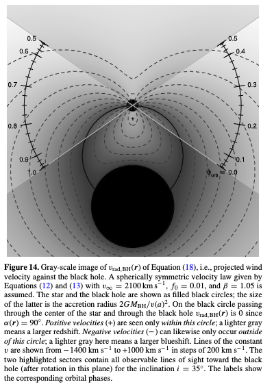
この記事では、Cygnus X-1 連星系における伴星からの星風の速度場を計算する Python プログラムを分解し、その重要な部分を解説します。特に、球対称星風モデルの基本式を用いた速度場の計算について、

で用いられた計算をベースに、速度場を描く例を紹介します。

具体的には、figure14 と同じ図を、python ベースで書く例に相当しています。

関連ページ

• ロッシュポテンシャルの書き方について

• Cyg X-1 の星風モデル (Gies, D. R., Bolton, C. T. 1986) について

---

1. 背景: 球対称星風モデル

球対称星風モデルでは、伴星表面から放出される風の速度を次の式で表現します。

$$
v(r) = v_{\infty} \cdot f\left(r / R_{\star}\right)
$$

ここで:

• $v_{\infty}$ は風の終端速度。
• $f(x)$ は終端速度に対する比率で、以下の式で与えられます (Lamers & Leitherer 1993):

$$
f(x) = f_0 + (1 - f_0) \cdot (1 - 1/x)^\beta \quad (\text{for } x \geqslant 1)
$$

このモデルでは、以下のパラメータが重要です。

• $f_0$: 星風の基底速度 $v_0$ と終端速度 $v_{\infty}$ の比率 $\left(f_0 = v_0 / v_{\infty}\right)$
• $\beta$: 星風の加速を決定する指数

---

2. 速度場の計算コード

次に、calculate_velocity_field 関数を詳しく解説します。

関数の概要

この関数は、与えられた2次元座標グリッドにおける伴星からの星風の速度場を計算します。

def calculate_velocity_field(X, Y, star_x, R_star, f0=0.01, beta=0.75, v_infty=2100, scale=1.0):

引数

• X, Y: 速度場を計算する2次元グリッドの座標
• star_x: 伴星の中心のX座標
• R_star: 伴星の半径
• f0: 基底速度の比率 (デフォルト値: 0.01)
• beta: 星風加速の指数 (デフォルト値: 0.75)
• v_infty: 終端速度 [km/s] (デフォルト値: 2100 km/s)
• scale: 距離単位のスケール (デフォルト値: 1.0)

出力

• Vx, Vy: 星風速度のX成分とY成分

---

主な計算の流れ

1. 距離の計算
   伴星中心から各グリッド点までの距離 $r$ を計算します。

   R_star_grid = np.sqrt((X - star_x)**2 + Y**2)
   

2. 正規化された距離
   $x = r / R_{\star}$ を計算し、$x \geq 1$ の点のみを対象に速度を計算します。

   x = R_star_grid / R_star_scaled
   mask = x >= 1
   

3. 速度の計算
   $f(x)$ を用いて星風速度 $v(r)$ を計算します。伴星内部 ($r < R_{\star}$) では速度を0に設定します。

   f_x[mask] = f0 + (1 - f0) * (1 - 1 / x[mask])**beta
   v_r = v_infty * f_x
   v_r[R_star_grid < R_star_scaled] = 0
   

4. 速度成分
   $v(r)$ を用いて、速度のX成分とY成分を計算します。

   Vx = v_r * (X - star_x) / R_star_grid
   Vy = v_r * Y / R_star_grid
   

5. 伴星内部の速度をゼロに
   恒星内部では速度成分をゼロに設定します。

   Vx[R_star_grid < R_star_scaled] = 0
   Vy[R_star_grid < R_star_scaled] = 0
   

---

3. プロット: Cyg X-1連星系の速度場

plot_binary_system_with_velocity 関数は、計算した速度場をプロットします。この関数では以下の3種類の速度場を可視化できます。

3.1 星風の全体的な速度場

• mode="star_wind"
• 星風が伴星から放射状に流れる様子を示します。

3.2 ブラックホール方向の速度成分

• mode="towards_bh"
• 星風の速度場のうち、ブラックホール方向の成分を抽出してプロットします。

3.3 垂直方向の速度成分

• mode="perpendicular_bh"
• ブラックホール方向に垂直な成分をプロットします。

---

4. 実行例

以下は、Cyg X-1連星系のデータを用いて速度場を計算し、プロットする例です。

# Cyg X-1 のデータ
period_days = 5.6  # 軌道周期 [日]
M_bh = 21.2 * M_sun  # ブラックホール質量 [kg]
M_star = 40.6 * M_sun  # 伴星質量 [kg]
R_star = 22.3 * SOLAR_RADIUS  # 伴星半径 [m]

# 軌道分離距離の計算
distance_cygx1 = calculate_mean_distance(M_bh, M_star, period_days)

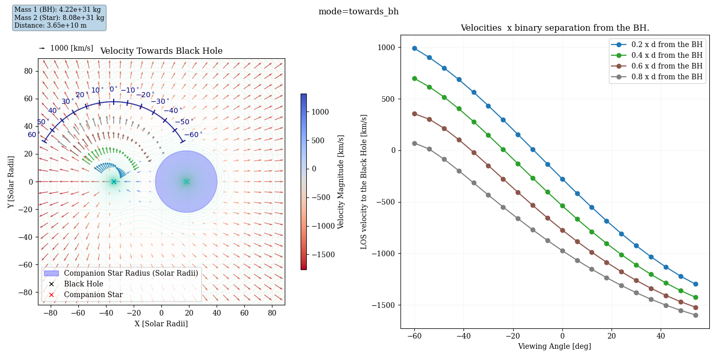
Subplot の説明: 左と右にプロットされた内容

左側のプロット: 速度場の可視化

左側のプロットでは、連星系における星風の速度場を描画しています。具体的には、以下の特徴を含みます:

1. 速度ベクトル:

   • 各グリッド点での星風の速度ベクトルが矢印で示されています。
   • 矢印の方向は速度の向きを、長さは速度の大きさを表します。

2. 速度の大きさの色付け:

   • 背景に速度の大きさ (スカラー場) がカラーマップとして表示されています。
   • 色の変化により、星風の強度が空間的にどのように分布しているかを直感的に理解できます。

3. 伴星とブラックホールの位置:

   • 伴星は赤い十字 (×) で、ブラックホールは黒い十字 (×) でプロットされています。
   • 伴星の半径を青い円として示し、星風の放出源であることを明示しています。

4. 等ポテンシャル線 (オプション):

   • ロッシュポテンシャルが計算されている場合、連星系の重力ポテンシャルの等高線が背景に追加されています。
   • 特に重力ポテンシャルの支配領域やロッシュローブを視覚的に確認できます。

右側のプロット: 視線速度のプロファイル

右側のプロットでは、星風の視線方向 (ブラックホール方向) の速度成分がプロファイルとして描画されています。

1. プロット内容:

   • 各距離 (ブラックホール中心から異なる半径) における視線速度の大きさがプロットされています。
   • 距離はブラックホールからの割合 (例: 0.2, 0.4, 0.6 倍の連星間距離) で示されます。

2. データ点:

   • 各プロットは、指定された距離における速度成分を、視線方向に対する見かけの角度 (度) に対してプロットしています。

3. 曲線のラベル:

   • 各曲線は、ブラックホールからの距離を明示するラベルが付けられており、異なる距離での視線速度の変化を比較できます。

4. 物理的意義:

   • このプロットにより、視線速度がブラックホール方向およびその周囲でどのように変化するかが定量的に解析できます。inclination が 約30度と言われてますが、それ以外の可能性もあるので、+/-60度の範囲で計算しています。
   • 特に、星風がブラックホールに向かう速度が最も大きくなる方向や、垂直方向の成分の変化を確認できます。

星風の速度場のプロット結果

• 球対称の星風の速度場のプロット

plot_binary_system_with_velocity(M_bh, M_star, R_star, distance_cygx1, mode="star_wind", unit="solar_radius")

• Cyg X-1 方向に射影したプロット

plot_binary_system_with_velocity(M_bh, M_star, R_star, distance_cygx1, mode="towards_bh", unit="solar_radius")

• Cyg X-1 方向に垂直な速度場のプロット

plot_binary_system_with_velocity(M_bh, M_star, R_star, distance_cygx1, mode="perpendicular_bh", unit="solar_radius")

---

コード全文

においています。

astro_plot_cygx1_wind.py

#!/usr/bin/env python 

import numpy as np
import matplotlib.pyplot as plt
plt.rcParams['font.family'] = 'serif'
from scipy.interpolate import RegularGridInterpolator
from matplotlib.colors import LogNorm

# 定数の定義
G = 6.67430e-11  # Gravitational constant [m^3 kg^-1 s^-2]
DAY_TO_SECOND = 86400  # Days to seconds conversion
M_sun = 1.989e30  # Solar mass [kg]
SOLAR_RADIUS = 6.957e8  # Solar radius [m]
# カラーマップを定義
cmap_forlines = plt.get_cmap('tab10')  # 好みのカラーマップを選択

def calculate_mean_distance(m1, m2, period_days):
    """
    Calculate the mean distance between two bodies in a binary system.

    Parameters
    ----------
    m1 : float
        Mass of the primary body [kg].
    m2 : float
        Mass of the secondary body [kg].
    period_days : float
        Orbital period of the system [days].

    Returns
    -------
    distance : float
        Mean distance between the two bodies [m].
    """
    period_seconds = period_days * DAY_TO_SECOND
    total_mass = m1 + m2
    distance = ((G * total_mass * period_seconds**2) / (4 * np.pi**2))**(1/3)
    print(f"Calculating mean distance for m1={m1:.2e} kg, m2={m2:.2e} kg, period={period_days} days, Mean distance: {distance:.2e} m")
    return distance

def calculate_velocity_field(X, Y, star_x, R_star, f0=0.01, beta=0.75, v_infty=2100, scale=1.0):
    """
    Calculate the velocity field of a stellar wind on a grid using the specified velocity law.

    Parameters
    ----------
    X : np.ndarray
        X-coordinates of the grid points [same unit as R_star].
    Y : np.ndarray
        Y-coordinates of the grid points [same unit as R_star].
    star_x : float
        X-coordinate of the companion star's center [same unit as R_star].
    R_star : float
        Radius of the companion star [same unit as grid].
    f0 : float, optional
        Fraction of the terminal velocity at the base of the wind. Default is 0.01.
    beta : float, optional
        Exponent of the velocity law. Default is 0.75.
    v_infty : float, optional
        Terminal velocity of the wind [km/s]. Default is 2100 km/s (2100e3 m/s).
    scale : float, optional
        Scaling factor to convert units (e.g., from meters to solar radii). Default is 1.0.

    Returns
    -------
    Vx : np.ndarray
        X-component of the velocity field (Default unit is [km/s]).
    Vy : np.ndarray
        Y-component of the velocity field (Default unit is [km/s]).
    """
    print(f"Calculating velocity field for star_x={star_x}, R_star={R_star} (scale={scale})...")
    # グリッド上の恒星からの距離を計算
    R_star_grid = np.sqrt((X - star_x)**2 + Y**2)
    R_star_scaled = R_star / scale  # 恒星の半径をスケール変換

    # 距離を正規化 (x = r / R_star)
    x = R_star_grid / R_star_scaled

    # f(x) の計算
    f_x = np.zeros_like(x)
    mask = x >= 1  # x >= 1 の条件を満たす点のみ計算
    f_x[mask] = f0 + (1 - f0) * (1 - 1 / x[mask])**beta

    # 星風の速度 v(r)
    v_r = v_infty * f_x

    # 恒星内部（r < R_star）で速度を 0 に設定
    v_r[R_star_grid < R_star_scaled] = 0

    # 速度場の X, Y 成分を計算
    Vx = v_r * (X - star_x) / R_star_grid
    Vy = v_r * Y / R_star_grid

    # 恒星内部（r < R_star）で速度成分を 0 に設定
    Vx[R_star_grid < R_star_scaled] = 0
    Vy[R_star_grid < R_star_scaled] = 0
    return Vx, Vy

def calculate_velocity_components(X, Y, Vx, Vy, bh_x, bh_y):
    """
    Calculate the velocity components in the direction of the black hole and perpendicular to it.

    Parameters
    ----------
    X : np.ndarray
        X-coordinates of the grid points.
    Y : np.ndarray
        Y-coordinates of the grid points.
    Vx : np.ndarray
        X-component of the velocity field.
    Vy : np.ndarray
        Y-component of the velocity field.
    bh_x : float
        X-coordinate of the black hole's position.
    bh_y : float
        Y-coordinate of the black hole's position.

    Returns
    -------
    V_bh_x : np.ndarray
        X-component of the velocity in the black hole's direction.
    V_bh_y : np.ndarray
        Y-component of the velocity in the black hole's direction.
    V_bh_magnitude : np.ndarray
        Magnitude of the velocity in the black hole's direction.
    V_perp_x : np.ndarray
        X-component of the velocity perpendicular to the black hole's direction.
    V_perp_y : np.ndarray
        Y-component of the velocity perpendicular to the black hole's direction.
    V_perp_magnitude : np.ndarray
        Magnitude of the velocity perpendicular to the black hole's direction.
    """
    # ブラックホール方向の単位ベクトル
    n_x = bh_x - X
    n_y = bh_y - Y
    n_mag = np.sqrt(n_x**2 + n_y**2)
    n_x /= n_mag
    n_y /= n_mag

    # ブラックホール方向の速度成分（符号付き）
    V_bh_magnitude = Vx * n_x + Vy * n_y
    V_bh_x = V_bh_magnitude * n_x
    V_bh_y = V_bh_magnitude * n_y

    # ブラックホール垂直方向の速度成分（符号付き）
    V_perp_x = Vx - V_bh_x
    V_perp_y = Vy - V_bh_y
    V_perp_magnitude = Vx * n_y - Vy * n_x  # 外積に基づいた符号付きの計算
    return V_bh_x, V_bh_y, V_bh_magnitude, V_perp_x, V_perp_y, V_perp_magnitude


def convert_angles_to_inclination(angles):
    """
    Convert angles in radians to inclination degrees with +π/2 as 0°.

    Parameters
    ----------
    angles : np.ndarray
        Array of angles in radians.

    Returns
    -------
    inclinations : np.ndarray
        Array of inclination angles in degrees, with +π/2 as 0°.
    """
    # Shift angles so +π/2 becomes 0 radians
    shifted_angles = angles - np.pi / 2

    # Convert radians to degrees
    inclinations = np.degrees(shifted_angles)

    return inclinations


def plot_arc_with_tics_on_axis(axis, center, radius, angles_degrees, tics_length=0.05, label_offset=0.2, offset_angle = 90.0):
    """
    Plot a circular arc with tics at specified angles on a given axis.

    Parameters
    ----------
    axis : matplotlib.axes.Axes
        The axis on which to plot the arc and tics.
    center : tuple
        Coordinates of the center of the arc (x, y).
    radius : float
        Radius of the arc.
    angles_degrees : list or np.ndarray
        List of angles in degrees where tics should be drawn.
    tics_length : float, optional
        Length of the tics, as a fraction of the radius. Default is 0.05.
    label_offset : float, optional
        Offset of the tic labels from the arc, as a fraction of the radius. Default is 0.1.
    """
    x_center, y_center = center

    # Create angles for the arc
    theta_arc = np.linspace(min(angles_degrees), max(angles_degrees), 500) +  offset_angle
    theta_arc_rad = np.radians(theta_arc)

    # Arc coordinates
    arc_x = x_center + radius * np.cos(theta_arc_rad)
    arc_y = y_center + radius * np.sin(theta_arc_rad)

    # Plot the arc on the specified axis
    axis.plot(arc_x, arc_y, color='navy', alpha=0.8)

    # Draw tics and labels
    for angle in angles_degrees:
        theta_rad = np.radians(angle +  offset_angle)
        # Start and end points of the tic
        tic_x_start = x_center + (radius - tics_length * radius) * np.cos(theta_rad)
        tic_y_start = y_center + (radius - tics_length * radius) * np.sin(theta_rad)
        tic_x_end = x_center + (radius + tics_length * radius) * np.cos(theta_rad)
        tic_y_end = y_center + (radius + tics_length * radius) * np.sin(theta_rad)

        # Draw the tic
        axis.plot([tic_x_start, tic_x_end], [tic_y_start, tic_y_end], color='navy', alpha=0.9)

        # Label position
        label_x = x_center + (radius + label_offset * radius) * np.cos(theta_rad) 
        label_y = y_center + (radius + label_offset * radius) * np.sin(theta_rad)

        # Add the label
        axis.text(label_x, label_y, f"${angle}^\circ$", ha='center', va='center', fontsize=10, color='navy')


def calculate_roche_potential(X, Y, m1, m2, distance):
    """
    Calculate the Roche potential for a binary system at given points (X, Y).

    Parameters
    ----------
    X : ndarray
        x-coordinates of the grid points [m].
    Y : ndarray
        y-coordinates of the grid points [m].
    m1 : float
        Mass of the primary body [kg].
    m2 : float
        Mass of the secondary body [kg].
    distance : float
        Distance between the centers of the two bodies [m].

    Returns
    -------
    potential : ndarray
        The Roche potential at each grid point [J/kg].
    """
    print("Calculating Roche potential...")
    mu = m2 / (m1 + m2)
    omega = np.sqrt(G * (m1 + m2) / distance**3)
    print(f"  Reduced mass parameter (mu): {mu:.5f}")
    print(f"  Orbital angular velocity (omega): {omega:.5e} [rad/s]")

    r1 = np.sqrt((X + mu * distance)**2 + Y**2)
    r2 = np.sqrt((X - (1 - mu) * distance)**2 + Y**2)
    potential = -G * m1 / r1 - G * m2 / r2 - 0.5 * omega**2 * (X**2 + Y**2)
    print("  Roche potential calculation completed.")
    return potential


def plot_binary_system_with_velocity(
    M_bh, M_star, R_star, distance_cygx1, grid_size=25, grid_range_factor=1.7, 
    v_scale=0.05, cmap='coolwarm_r', plot_star_radius=True, mode="star_wind", unit="m", plot_roche=True):
    """
    Visualize the velocity field of a binary system with a black hole and a companion star.

    Parameters
    ----------
    M_bh : float
        Mass of the black hole [kg].
    M_star : float
        Mass of the companion star [kg].
    R_star : float
        Radius of the companion star [unit determined by `unit`].
    distance_cygx1 : float
        Orbital separation between the black hole and the companion star [unit determined by `unit`].
    grid_size : int, optional
        Number of grid points along each axis for plotting the velocity field. Default is 30.
    grid_range_factor : float, optional
        Factor to scale the grid range relative to the orbital separation. Default is 1.7.
    v_scale : float, optional
        Scale factor for the velocity vector arrows. Default is 0.05.
    cmap : str, optional
        Colormap to use for the velocity magnitude visualization. Default is 'coolwarm_r'.
    plot_star_radius : bool, optional
        Whether to visualize the companion star's radius on the plot. Default is True.
    mode : str, optional
        Mode of the velocity field to visualize. Choose from:
        - "star_wind": Radial velocity field originating from the star.
        - "towards_bh": Velocity field component directed toward the black hole.
        - "perpendicular_bh": Velocity field component perpendicular to the black hole direction.
        Default is "star_wind".
    unit : str, optional
        Unit of distance to use for the plot. Choose from:
        - "m": Meters.
        - "solar_radius": Solar radii.
        Default is "m".

    Returns
    -------
    None
        The function generates and displays a plot, and saves it as a PNG file.
    """
    print(f"Starting plot for mode={mode}, unit={unit}...")
    # 単位スケーリングとラベル設定
    if unit == "solar_radius":
        scale = SOLAR_RADIUS
        unit_label = "Solar Radii"
    elif unit == "m":
        scale = 1.0
        unit_label = "Meters"
    else:
        raise ValueError("Invalid unit. Choose 'm' or 'solar_radius'.")

    # 共通重心を原点とした座標系での位置（単位変換を適用）
    bh_x = -distance_cygx1 * (M_star / (M_bh + M_star)) / scale
    bh_y = 0
    star_x = distance_cygx1 * (M_bh / (M_bh + M_star)) / scale

    # 描画範囲
    grid_range = grid_range_factor * distance_cygx1 / scale
    x = np.linspace(-grid_range, grid_range, grid_size)
    y = np.linspace(-grid_range, grid_range, grid_size)
    X, Y = np.meshgrid(x, y)

    # 伴星からの距離 r を計算
    R_star_grid = np.sqrt((X - star_x)**2 + Y**2)
    R_star_scaled = R_star / scale  # 半径の単位変換

    # 速度場を計算
    Vx, Vy = calculate_velocity_field(X, Y, star_x, R_star, scale=scale)

    # ブラックホール方向の速度成分（符号付き）、垂直方向の速度成分（符号付き）の計算
    V_bh_x, V_bh_y, V_bh_magnitude, V_perp_x, V_perp_y, V_perp_magnitude = calculate_velocity_components(X, Y, Vx, Vy, bh_x, bh_y)

    # プロットする速度場を選択
    if mode == "star_wind":
        plot_Vx, plot_Vy, plot_Vmag, title, cmap = Vx, Vy, np.sqrt(Vx**2 + Vy**2), "Star Wind Velocity Field", "Reds"
        filename = f"cygx1_star_wind_velocity_{unit}.png"
    elif mode == "towards_bh":
        plot_Vx, plot_Vy, plot_Vmag, title = V_bh_x, V_bh_y, V_bh_magnitude, "Velocity Towards Black Hole"
        filename = f"cygx1_towards_bh_velocity_{unit}.png"
    elif mode == "perpendicular_bh":
        plot_Vx, plot_Vy, plot_Vmag, title = V_perp_x, V_perp_y, V_perp_magnitude, "Perpendicular Velocity Field"
        filename = f"cygx1_perpendicular_bh_velocity_{unit}.png"
    else:
        raise ValueError(f"Invalid mode: {mode}. Choose from 'star_wind', 'towards_bh', 'perpendicular_bh'.")

    desired_arrow_length = x[1] - x[0]  # minimum grid size of x is used for the max value of the arrow 
    max_velocity = np.max(np.sqrt(plot_Vx**2 + plot_Vy**2))
    arrow_scale = max_velocity / desired_arrow_length
    print(f"arrow_scale = {arrow_scale}, max_velocity = {max_velocity},  desired_arrow_length = {desired_arrow_length}")

    ############# plot ######################################
    nrows, ncols = 1, 2 
    fig, axes = plt.subplots(figsize=(14, 7), nrows=nrows, ncols=ncols, tight_layout=True)
    angles_num_points=20    
    angles = np.linspace(+np.pi/6, +5*np.pi/6, angles_num_points, endpoint=False)
    inclinations = convert_angles_to_inclination(angles)    

    # 伴星の半径を描画
    if plot_star_radius:
        circle = plt.Circle(
            (star_x, 0),  # 中心座標
            R_star_scaled,  # 半径
            color='blue',
            alpha=0.3,
            label=f"Companion Star Radius ({unit_label})"
        )
        axes[0].add_artist(circle)

    plt.suptitle(f"mode={mode}")
    # 描画設定
    axes[0].set_xlim(-grid_range, grid_range)
    axes[0].set_ylim(-grid_range, grid_range)
    axes[0].set_aspect('equal')
    axes[0].set_title(title)
    axes[0].set_xlabel(f"X [{unit_label}]")
    axes[0].set_ylabel(f"Y [{unit_label}]")
    axes[0].grid(alpha=0.1)

    # plot BH and star
    axes[0].plot(bh_x, 0, 'kx', markersize=6, label='Black Hole')  # ブラックホール
    axes[0].plot(star_x, 0, 'rx', markersize=6, label='Companion Star')  # 伴星

    # 結果のプロット
    quiver = axes[0].quiver(
        X, Y, plot_Vx, plot_Vy, plot_Vmag,
        cmap=cmap, scale=arrow_scale, scale_units='xy', angles='xy'
    )
    # 矢印のスケール説明を追加
    quiver_scale_length = 1000  # 矢印のスケール基準 (速度の大きさが quiver_scale_length のときの矢印の長さ)
    quiver_key = axes[0].quiverkey(
        quiver, X=0.03, Y=1.04, U=quiver_scale_length, label=f"{quiver_scale_length} [km/s]",
        labelpos='E', coordinates='axes'
    )
    # Colorbar
    cbar = plt.colorbar(quiver, ax=axes[0], shrink=0.6, aspect=30)
    cbar.set_label('Velocity Magnitude [km/s]')

    arc_center = (bh_x, bh_y)  # ブラックホールを中心
    arc_radius = 1.1 * distance_cygx1 / scale

    # 最大角度とステップを指定
    max_angle = 60  # 最大角度
    step = 10       # ステップ    
    angles_degrees = list(range(-max_angle, max_angle + 1, step))

    plot_arc_with_tics_on_axis(axes[0], arc_center, arc_radius, angles_degrees, tics_length=0.03, label_offset=0.15)

    axes[1].set_xlabel("Viewing Angle [deg]")
    axes[1].set_ylabel("LOS velocity to the Black Hole [km/s]")
    axes[1].set_title("Velocities  x binary separation from the BH.")
    axes[1].grid(alpha=0.1)

    if plot_roche:
        # need to prepare find grid to plot smooth potential 
        x = np.linspace(-grid_range, grid_range, grid_size*10)
        y = np.linspace(-grid_range, grid_range, grid_size*10)
        X, Y = np.meshgrid(x, y)

        # Calculate Roche potential
        Z = calculate_roche_potential(X * scale, Y * scale, M_bh, M_star, distance_cygx1)
        Z_posi = -Z
        print("  Plotting the Roche potential...")

        contour_levels=100
        contour_levels_line=100
        levels = np.logspace(np.log10(Z_posi.min()), np.log10(Z_posi.max()), contour_levels)
        contour = axes[0].contourf(X, Y, Z_posi, levels=levels, cmap='Oranges', norm=LogNorm(), alpha=0.1)
        # add coutour 
        levels_line = np.logspace(np.log10(Z_posi.min()), np.log10(Z_posi.max()), contour_levels_line)    
        axes[0].contour(X, Y, Z_posi, levels=levels_line, colors="cyan", linewidths=0.5, alpha=0.2)


    for idx, proj_fraction in enumerate([0.2,0.4,0.6,0.8]):
        # カラーマップから色を取得
        color = cmap_forlines(idx / 4.0)  # 0.2, 0.4, 0.6, 0.8 に基づく色        
        # # ブラックホールから一定距離 r の円周上の点列に対して速度場を求める
        proj_radius = proj_fraction * distance_cygx1 / scale
        # 角度を反時計回りで等間隔に円周上の点を計算
        points = np.array([
            (bh_x + proj_radius * np.cos(theta), bh_y + proj_radius * np.sin(theta)) for theta in angles
        ])
        # 速度場を計算
        proj_Vx, proj_Vy = calculate_velocity_field(points.T[0], points.T[1], star_x, R_star, scale=scale)
        proj_V_bh_x, proj_V_bh_y, proj_V_bh_magnitude, proj_V_perp_x, proj_V_perp_y, proj_V_perp_magnitude = \
        calculate_velocity_components(points.T[0], points.T[1], proj_Vx, proj_Vy, bh_x, bh_y)

        # プロットする速度場を選択
        if mode == "star_wind":
            proj_plot_Vx, proj_plot_Vy, proj_Vmag, title, cmap = proj_Vx, proj_Vy, np.sqrt(proj_Vx**2 + proj_Vy**2), "Star Wind Velocity Field", "Reds"
            filename = f"check_vfields_cygx1_star_wind_velocity_{unit}.png"
        elif mode == "towards_bh":
            proj_plot_Vx, proj_plot_Vy, proj_Vmag, title = proj_V_bh_x, proj_V_bh_y, proj_V_bh_magnitude, "Velocity Towards Black Hole"
            filename = f"check_vfields_cygx1_towards_bh_velocity_{unit}.png"
        elif mode == "perpendicular_bh":
            proj_plot_Vx, proj_plot_Vy, proj_Vmag, title = proj_V_perp_x, proj_V_perp_y, proj_V_perp_magnitude, "Perpendicular Velocity Field"
            filename = f"check_vfields_cygx1_perpendicular_bh_velocity_{unit}.png"
        else:
            raise ValueError(f"Invalid mode: {mode}. Choose from 'star_wind', 'towards_bh', 'perpendicular_bh'.")

        for i, (x, y) in enumerate(points):            
            axes[0].arrow(x, y, proj_plot_Vx[i]/arrow_scale, proj_plot_Vy[i]/arrow_scale, head_width=1, head_length=1, color=color,alpha=0.8)

        axes[1].plot(inclinations, proj_Vmag, 'o-', color=color, markersize=6, label=f"{proj_fraction} x d from the BH")
        axes[1].legend()

    axes[0].legend()

    # Optionally display plot details
    detail_text = (
        f"Mass 1 (BH): {M_bh:.2e} kg\n"
        f"Mass 2 (Star): {M_star:.2e} kg\n"
        f"Distance: {distance_cygx1:.2e} m"
    )
    fig.text(0.02, 0.95, detail_text, fontsize=9, va="center", ha="left", bbox=dict(boxstyle="round", alpha=0.3))


    plt.savefig(f"{filename}")
    print(f"Plot saved as {filename}")
    plt.show()

# Cyg X-1 のデータを使用
period_days = 5.6  # Orbital period [days]
M_bh = 21.2 * M_sun  # Black hole mass [kg]
M_star = 40.6 * M_sun  # Companion star mass [kg]
R_star = 22.3 * SOLAR_RADIUS  # Companion star radius [m]

# 平均距離を計算
distance_cygx1 = calculate_mean_distance(M_bh, M_star, period_days)

# 実行例
print("***** Plot velocity field for stellar wind *****" )
plot_binary_system_with_velocity(M_bh, M_star, R_star, distance_cygx1, mode="star_wind", unit="solar_radius")
print("\n***** Plot velocity field for stellar wind parallel to BH *****" )
plot_binary_system_with_velocity(M_bh, M_star, R_star, distance_cygx1, mode="towards_bh", unit="solar_radius")  # 視線方向
print("\n***** Plot velocity field for stellar wind vertical to BH *****" )
plot_binary_system_with_velocity(M_bh, M_star, R_star, distance_cygx1, mode="perpendicular_bh", unit="solar_radius")  # 垂直方向

5. 結論

このプログラムは、球対称星風モデルを基にCyg X-1連星系の詳細な速度場を計算し、可視化するツールです。このコードを応用すれば、他の連星系や条件下での星風の挙動を解析することも可能です。