HR図を astroquery と Google Colab で描こう:距離補正と温度換算までやってみる
ヘルツシュプルング・ラッセル図(HR図)は、星の明るさと温度の関係を示す天文学の基本図です。
この記事では、astroquery を使って、ヒッパルコス衛星カタログの実データから ヘルツシュプルング・ラッセル図(HR図)を描き、距離補正(絶対等級化)と温度換算まで行います。
Google Colab 上で簡単に実行できるので、天文データ解析の第一歩としてまずは遊んでみましょう!
👉 Colab 実行用ノートブックはこちら
🧭 この記事で学べること
| ステップ | 内容 |
|---|---|
| 1 | astroquery で天文データを取得する方法 |
| 2 | 視差から距離を求める(パーセク換算) |
| 3 | HR図(見かけ等級)をプロット |
| 4 | 距離補正して絶対等級に変換 |
| 5 | B−V から有効温度を推定して物理的HR図を描く |
🧩 Step 1: astroquery のインストール
Google Colab の最初のセルに以下を入力します。
!pip install astroquery
astroquery は、NASA や ESA などの天文データベース(Vizier, SIMBAD, Gaiaなど)にアクセスするための Python ライブラリです。
🧩 Step 2: データを取得して中身を確認する
from astroquery.vizier import Vizier
import numpy as np
import matplotlib.pyplot as plt

# ヒッパルコス主カタログ (I/239/hip_main)
v = Vizier(
    catalog="I/239/hip_main",
    columns=["HIP", "Vmag", "B-V", "Plx"],
    row_limit=-1
)

data = v.query_constraints()
tbl = data[0]

# 各列を抽出
vmag = tbl["Vmag"]   # Vバンドの見かけ等級
bv   = tbl["B-V"]    # 色指数 (B−V)
plx  = tbl["Plx"]    # 視差 [mas]

print("データ件数:", len(tbl))
print(tbl[:5])
🔍 データの意味
| 列名 | 内容 | 単位 |
|---|---|---|
| Vmag | 見かけ等級(地球から見た明るさ) | mag |
| B−V | 青色と可視光の明るさの差。温度の指標 | mag |
| Plx | 年周視差(距離の逆数) | ミリ秒角 (mas) |
🧩 Step 3: 視差から距離を求める
視差 ( p ) [mas] と距離 ( d ) [pc] の関係は以下の式で与えられます:
d = \frac{1}{p(\text{arcsec})} = \frac{1000}{p(\text{mas})}
def plx_to_parsec(marcsec):
    return 1.0 / (1e-3 * marcsec)

distance_pc = plx_to_parsec(plx)
print("距離範囲:", np.nanmin(distance_pc), "〜", np.nanmax(distance_pc), "pc")
🧩 Step 4: 距離が近い星で HR 図を描く
まず、距離がほぼ一定(40〜50 pc)にある星だけを選び、見かけ等級で HR 図を描いてみます。
pmin, pmax = 20, 25  # 視差 [mas]
mask = (plx > pmin) & (plx < pmax)

vmag_cut = vmag[mask]
bv_cut   = bv[mask]

plt.figure(figsize=(6,5))
plt.title("HR図(d ≈ 40–50 pc)")
plt.scatter(bv_cut, -vmag_cut, s=1)
plt.xlim(-0.1, 2)
plt.ylim(-13, 0)
plt.xlabel("B−V (色指数)")
plt.ylabel("−Vmag(明るい星ほど上)")
plt.grid(alpha=0.3)
plt.show()
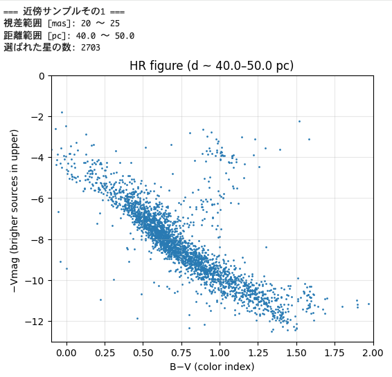
💬 ここでのポイント
- 主系列星が斜めの帯として現れます。
- 距離を固定したため、見かけ等級がほぼ「星そのものの明るさ」を反映します。
🧩 Step 5: 距離範囲を広げて比較してみよう
pmin, pmax = 5, 60  # 視差を広く取る(5〜60 mas)
mask = (plx > pmin) & (plx < pmax)
vmag_cut = vmag[mask]
bv_cut   = bv[mask]

plt.figure(figsize=(6,5))
plt.title("HR図(d ≈ 17〜200 pc)")
plt.scatter(bv_cut, -vmag_cut, s=1)
plt.xlim(-0.1, 2)
plt.ylim(-13, 0)
plt.xlabel("B−V (色指数)")
plt.ylabel("−Vmag")
plt.grid(alpha=0.3)
plt.show()
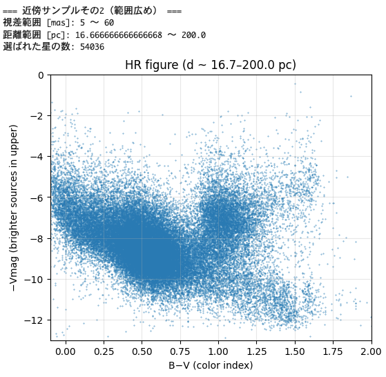
🧠 比較してみよう
- 星がバラけて見えるのは、距離が異なるため。
- これを補正するのが「絶対等級」です。
🧩 Step 6: 絶対等級に変換する(距離補正)
距離 (d) [pc] から絶対等級 (M_V) への変換式:
M_V = V - 5 \log_{10}(d / 10)
mask = (plx > 10) & (plx < 100)
distance_sel = distance_pc[mask]
bv_sel = bv[mask]
vmag_sel = vmag[mask]

abs_mag = vmag_sel - 5 * np.log10(distance_sel / 10)

plt.figure(figsize=(6,5))
plt.scatter(bv_sel, abs_mag, s=1)
plt.gca().invert_yaxis()
plt.xlabel("B−V (色指数)")
plt.ylabel("絶対等級 Mv")
plt.title("HR図(距離補正済み:絶対等級)")
plt.grid(alpha=0.3)
plt.show()
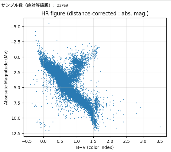
💡 絶対等級は「星が10 pcの距離にあるとしたときの明るさ」。
距離の違いが除かれ、星の本来の明るさの違いが見えてきます。
🧩 Step 7: B−V から温度に換算する
色指数 B−V は星の表面温度 ($T_{\mathrm{eff}}$) の指標になります。
簡易近似式(Ballesteros 2012)を使って温度を求めます。
T_{\mathrm{eff}} = 4600 \left( \frac{1}{0.92(B-V)+1.7} + \frac{1}{0.92(B-V)+0.62} \right)
def bv_to_temp(bv_value):
    return 4600 * ((1/(0.92*bv_value+1.7)) + (1/(0.92*bv_value+0.62)))

temp_sel = bv_to_temp(bv_sel)

plt.figure(figsize=(6,5))
plt.scatter(temp_sel, abs_mag, s=1)
plt.xscale("log")
plt.gca().invert_xaxis()
plt.gca().invert_yaxis()
plt.xlabel("有効温度 Teff [K]")
plt.ylabel("絶対等級 Mv")
plt.title("HR図(温度スケール)")
plt.grid(alpha=0.3)
plt.show()
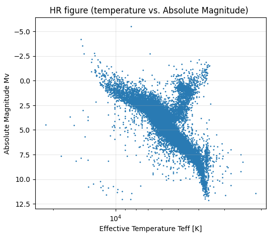
🌟 これが「教科書に出てくる本来の HR 図」!
左上:高温・明るい星(O型・B型)
右下:低温・暗い星(M型・赤色矮星)
左下:白色矮星の領域
🧩 Step 8: 発展課題
- 太陽の絶対等級 ( $M_\odot = 4.83$ ) を使って光度に換算し、
として、光度–温度図を描いてみよう。
\frac{L}{L_\odot} = 10^{-0.4(M - 4.83)} - 観測誤差(視差や等級の不確かさ)を考慮すると、どのようにばらつきが変わるか?
- Gaia DR3 カタログを使って同様の図を描き、分解能の違いを比べよう。
🪐 まとめ
| 段階 | 学べたこと |
|---|---|
| astroquery | 実際の星のデータを取得できる |
| 視差 → 距離 | 幾何学的に距離を求める原理 |
| 見かけ等級 vs 絶対等級 | 距離補正の意味を理解 |
| 色指数 → 温度 | 星の色と温度の関係を定量的に理解 |
| HR図の物理的意味 | 恒星の進化段階(主系列・巨星・矮星)を視覚的に把握 |
🔗 参考文献・リンク
- astroquery ドキュメント
- VizieR Catalog I/239/hip_main
- Ballesteros, F. J. (2012), Eur. J. Phys., 33, 1307. DOI: 10.1088/0143-0807/33/6/044
- Pythonでastroqueryを用いた銀河カタログの可視化(Qiita記事)
🚀 おわりに
このノートは、 「星の色・明るさ・距離」 という観測量を結びつけて理解する実習題材です。
最初は単なる散布図に見えるかもしれませんが、少しずつ補正・変換を加えることで「宇宙の物理的構造」が浮かび上がってきます。