はじめに
制限3体問題の基礎的な例として、ロッシュポテンシャルとラグランジュ点について、python で簡単に計算する方法を紹介します。
背景物理
ロッシュポテンシャルとは
ロッシュポテンシャルは、連星系や惑星系の2体間に働く重力、遠心力を合わせた有効ポテンシャルを表します。このポテンシャルを用いることで、質量中心に対する運動や、物体が引き寄せられる領域を解析することができます。ロッシュポテンシャル $\Phi$ は以下の式で定義されます:
\Phi(x, y) = -\frac{G M_1}{r_1} - \frac{G M_2}{r_2} - \frac{1}{2} \omega^2 (x^2 + y^2)
- $G$: 重力定数
- $M_1, M_2$: 主星と伴星の質量
- $r_1, r_2$: 各星からの距離
- $\omega$: 系の角速度
ロッシュポテンシャルは、原点を重心にとるか、どちらかの星にとるか、により表式が異なります。また無次元ロッシュポテンシャル(ロッシュポテンシャルをポテンシャルの次元(GM/R)で規格化したものを用いる場合も、表式が異なります。
ラグランジュ点 L1, L2, L3 の導出方法
ラグランジュ点 L1, L2, L3 は主星 $M_1$ と伴星 $M_2$ を結ぶ直線上に存在し、ロッシュポテンシャルの $x$ 軸方向の勾配がゼロとなる点として定義されます。
ロッシュポテンシャル $\Phi(x, y)$ の $x$ 軸勾配 $\frac{\partial \Phi}{\partial x}$ を計算すると、以下の式が得られます:
\frac{\partial \Phi}{\partial x} =
-\frac{G M_1 (x + \mu d)}{r_1^3}
-\frac{G M_2 (x - (1-\mu) d)}{r_2^3}
+ \omega^2 x
ここで、
- $r_1 = \sqrt{(x + \mu d)^2 + y^2}$: 主星 $M_1$ からの距離
- $r_2 = \sqrt{(x - (1-\mu) d)^2 + y^2}$: 伴星 $M_2$ からの距離
- $\mu = \frac{M_2}{M_1 + M_2}$: 無次元化した質量比
- $d$: 星間距離
- $\omega = \sqrt{\frac{G (M_1 + M_2)}{d^3}}$: 系の角速度
直線上 ($y = 0$) に限定すると、以下の式を得ます:
\frac{\partial \Phi}{\partial x} =
-\frac{G M_1 (x + \mu d)}{|x + \mu d|^3}
-\frac{G M_2 (x - (1-\mu) d)}{|x - (1-\mu) d|^3}
+ \omega^2 x = 0
式の無次元化
計算を簡略化するため、$GM/d$(ポテンシャルの次元)でポテンシャルを規格化し無次元ロッシュポテンシャルを考えます。式としては、$\Phi = \Phi/(GM/d)$ とする。これにより、$\Phi$と$x$は無次元化され、式は次のように簡略化されます:
\frac{\partial \Phi}{\partial x} =
(1 - \mu) \frac{x + \mu}{|x + \mu|^3}
+ \mu \frac{x - (1-\mu)}{|x - (1-\mu)|^3}
- x = 0
数値解法
この非線形方程式を解くために、Python の scipy.optimize.fsolve を用います。
初期値として以下を設定します:
- L1 近辺: $x = 0.5 - \mu$
- L2 近辺: $x = 1.5 - \mu$
- L3 近辺: $x = -1.5 - \mu$
具体的なコードは以下のとおりです:
def grad_potential_x(x, y, mu):
    r1 = np.sqrt((x + mu)**2 + y**2)
    r2 = np.sqrt((x - (1 - mu))**2 + y**2)
    return (1 - mu) * (x + mu) / r1**3 + mu * (x - (1 - mu)) / r2**3 - x

def find_lagrange_points(mu):
    guesses = [0.5 - mu, 1.5 - mu, -1.5 - mu]
    lagrange_points = []
    for guess in guesses:
        sol = fsolve(lambda x: grad_potential_x(x, 0, mu), guess)
        lagrange_points.append(sol[0])
    return lagrange_points
fsolve はニュートン法に基づき、初期値から収束的に解を求めます。結果として、無次元化された $x$ 座標が得られます。
L4, L5 の導出方法
数学的背景
L4, L5 は主星 $M_1$ と伴星 $M_2$ を結ぶ線を底辺とする正三角形の頂点に位置します。この配置を幾何学的に考慮すると、L4, L5 の位置は以下で表されます:
x = \frac{1}{2} - \mu, \quad y = \pm \frac{\sqrt{3}}{2}
無次元化の前提
この結果は、星間距離 $d$ を単位長さ ($d = 1$) とした場合にのみ成り立つことに注意してください。もし無次元化を行わない場合、L4, L5 の位置は以下のようになります:
x = \frac{1}{2}d - \mu d, \quad y = \pm \frac{\sqrt{3}}{2}d
つまり、距離 $d$ のスケールで変化します。無次元化の有無によって結果が異なります。
解法まとめ
| ラグランジュ点 | 数値解法または幾何学的解法 |
|---|---|
| L1, L2, L3 | 数値解法(fsolve) |
| L4, L5 | 幾何学的解法 |
プログラムと数値解法の解説
L1, L2, L3 の位置を計算する際、式の初期値や数値解法の設定が収束性に影響します。また、L4, L5 の解析解は無次元化された場合は単純な数値で表せます。原点の取り方や、無次元化、これらの点を誤解しないように計算結果を解釈することが大切です。
コリオリ力とポテンシャルの関係
コリオリ力とは
コリオリ力は、回転座標系で運動する物体に働く見かけの力で、物体の速度に比例して以下の形で表されます:
\mathbf{F}_\text{Coriolis} = -2 m (\boldsymbol{\omega} \times \mathbf{v})
- $m$: 質量
- $\boldsymbol{\omega}$: 回転座標系の角速度ベクトル
- $\mathbf{v}$: 回転座標系での物体の速度
この力は速度 $\mathbf{v}$ に依存するため、ポテンシャル関数を定義することができません。ポテンシャルは空間上の位置($\mathbf{r}$)のみに依存するスカラー量である必要があるためです。
ポテンシャルとして扱える力
ロッシュポテンシャルでは、コリオリ力以外の2つの力、重力と遠心力が扱われます。これらは次のようにポテンシャル関数の形で表すことが可能です:
-
重力ポテンシャル(各星の引力):
\Phi_\text{gravity} = -\frac{G M_1}{r_1} - \frac{G M_2}{r_2}- $r_1, r_2$: 主星 $M_1$ および伴星 $M_2$ からの距離
-
遠心力のポテンシャル(回転座標系の見かけの力):
\Phi_\text{centrifugal} = -\frac{1}{2} \omega^2 (x^2 + y^2)- $\omega$: 回転座標系の角速度
これらを足し合わせることで、ロッシュポテンシャルが定義されます:
\Phi(x, y) = -\frac{G M_1}{r_1} - \frac{G M_2}{r_2} - \frac{1}{2} \omega^2 (x^2 + y^2)
運動を考える場合
物体がポテンシャル面に沿って運動する場合、コリオリ力を考慮する必要があります。回転座標系では、運動方程式に次のような形でコリオリ力が加わります:
m \frac{d\mathbf{v}}{dt} = -\nabla \Phi + \mathbf{F}_\text{Coriolis}
ここで、
- $-\nabla \Phi$: ポテンシャルから導かれる力(重力と遠心力による成分)
- $\mathbf{F}_\text{Coriolis}$: コリオリ力(速度依存)
静的解析(ラグランジュ点の導出)におけるコリオリ力の不要性
ラグランジュ点の解析では、物体が静止している(見かけ上動いていない)状態を考えます。このとき速度 $\mathbf{v} = 0$ なので、コリオリ力はゼロになります:
\mathbf{F}_\text{Coriolis} = -2 m (\boldsymbol{\omega} \times \mathbf{v}) = 0
したがって、静的なラグランジュ点を求める際には、重力と遠心力のポテンシャルだけを考えれば十分です。ポテンシャル関数 $\Phi(x, y)$ の勾配がゼロになる点を探せば、ラグランジュ点が得られます。
- コリオリ力は速度に依存するためポテンシャル関数として表すことができません。
- ラグランジュ点の導出では、物体が静止している状態を仮定するため、コリオリ力は無視できます。
- ポテンシャルには重力と遠心力の寄与のみを含めることで、ラグランジュ点を特定することが可能です。
この違いを理解すると、動的解析と静的解析のそれぞれで必要な物理量が理解できます。
プログラムの解説
プロットの流れ
- グリッド作成
- ロッシュポテンシャル計算
- 等高線プロット
- ラグランジュ点のプロット
- 星や質量中心の描画
コード全文
においてあります。以下はコードの全文です。
#!/usr/bin/env python

import numpy as np
import matplotlib.pyplot as plt
plt.rcParams['font.family'] = 'serif'
from scipy.optimize import fsolve
from matplotlib.colors import LogNorm
import math
# 定数
G = 6.67430e-11  # 重力定数 [m^3/kg/s^2]
AU = 1.496e11  # 天文単位 [m]
SOLAR_RADIUS = 6.957e8  # 太陽半径 [m]
DAY_TO_SECOND = 86400  # 1日を秒に変換

def grad_potential_x(x, y, mu):
    """
    Calculate the x-component of the gradient of the Roche potential.

    Parameters
    ----------
    x : float
        x-coordinate [m].
    y : float
        y-coordinate [m].
    mu : float
        Reduced mass parameter (mass ratio of the secondary body).

    Returns
    -------
    gradient : float
        The x-component of the gradient of the Roche potential.
    """
    r1 = np.sqrt((x + mu)**2 + y**2)
    r2 = np.sqrt((x - (1 - mu))**2 + y**2)
    return (1 - mu) * (x + mu) / r1**3 + mu * (x - (1 - mu)) / r2**3 - x

def find_lagrange_points(mu):
    """
    Calculate the positions of the Lagrange points (L1, L2, L3).

    Parameters
    ----------
    mu : float
        Reduced mass parameter (mass ratio of the secondary body).

    Returns
    -------
    lagrange_points : list of float
        Positions of L1, L2, and L3 along the x-axis [m].
    """
    print("Finding Lagrange points...")
    guesses = [0.5 - mu, 1.5 - mu, -1.5 - mu]
    lagrange_points = []
    for guess in guesses:
        sol = fsolve(lambda x: grad_potential_x(x, 0, mu), guess)
        lagrange_points.append(sol[0])
        print(f"  Initial guess: {guess:.2f}, Lagrange point: {sol[0]:.5e} [m]")
    return lagrange_points

def calculate_mean_distance(m1, m2, period_days):
    """
    Calculate the mean distance between two bodies in a binary system.

    Parameters
    ----------
    m1 : float
        Mass of the primary body [kg].
    m2 : float
        Mass of the secondary body [kg].
    period_days : float
        Orbital period of the system [days].

    Returns
    -------
    distance : float
        Mean distance between the two bodies [m].
    """
    print(f"Calculating mean distance for orbital period: {period_days} days")
    period_seconds = period_days * DAY_TO_SECOND
    total_mass = m1 + m2
    distance = ((G * total_mass * period_seconds**2) / (4 * np.pi**2))**(1/3)
    print(f"  Mean distance: {distance:.5e} [m]")
    return distance

def calculate_roche_potential(X, Y, m1, m2, distance):
    """
    Calculate the Roche potential for a binary system at given points (X, Y).

    Parameters
    ----------
    X : ndarray
        x-coordinates of the grid points [m].
    Y : ndarray
        y-coordinates of the grid points [m].
    m1 : float
        Mass of the primary body [kg].
    m2 : float
        Mass of the secondary body [kg].
    distance : float
        Distance between the centers of the two bodies [m].

    Returns
    -------
    potential : ndarray
        The Roche potential at each grid point [J/kg].
    """
    print("Calculating Roche potential...")
    mu = m2 / (m1 + m2)
    omega = np.sqrt(G * (m1 + m2) / distance**3)
    print(f"  Reduced mass parameter (mu): {mu:.5f}")
    print(f"  Orbital angular velocity (omega): {omega:.5e} [rad/s]")

    r1 = np.sqrt((X + mu * distance)**2 + Y**2)
    r2 = np.sqrt((X - (1 - mu) * distance)**2 + Y**2)
    potential = -G * m1 / r1 - G * m2 / r2 - 0.5 * omega**2 * (X**2 + Y**2)
    print("  Roche potential calculation completed.")
    return potential


def plot_physical_potential(
    m1, m2, distance, unit="m", star_radius=None, plot_center=False, title=None,
    savefig=None, plot_detail=True, contour_levels=50, contour_levels_line=50, star_radius_tangent=False
):
    """
    Plot the Roche potential and the positions of the Lagrange points.
    Optionally display additional details, centers, and save the plot.

    Parameters
    ----------
    m1 : float
        Mass of the primary body [kg].
    m2 : float
        Mass of the secondary body [kg].
    distance : float
        Distance between the two bodies [m].
    unit : str, optional
        Unit for the plot axes ('m', 'AU', or 'solar_radius'). Default is 'm'.
    star_radius : float, optional
        Radius of the secondary star [m]. If specified, a circle representing the star is plotted.
    plot_center : bool, optional
        If True, marks the positions of the centers (m1, m2) and the barycenter.
    title : str, optional
        Title of the plot. If None, no title is set.
    savefig : str, optional
        Path to save the figure. If None, the plot is not saved.
    plot_detail : bool, optional
        If True, displays additional details (masses, distance, etc.) on the plot.
    contour_levels : int, optional
        Number of levels for the contour plot. Default is 50.
    contour_levels_line : int, optional
        Number of levels for the contour plot for a line style. Default is 50.
    star_radius_tangent : bool, optional
        If True, plot tangential lines at the star surface

    Raises
    ------
    ValueError
        If an invalid unit is provided.
    """
    print("Starting Roche potential plot...")
    print("  Coordinate system origin: barycenter of the system.")

    # Unit conversion
    units_conversion = {"m": 1, "AU": AU, "solar_radius": SOLAR_RADIUS}
    if unit not in units_conversion:
        raise ValueError(f"Invalid unit: {unit}. Choose from {list(units_conversion.keys())}.")

    scale = units_conversion[unit]
    mu = m2 / (m1 + m2)

    # Create grid
    x = np.linspace(-1.5 * distance, 1.5 * distance, 500) / scale
    y = np.linspace(-1.5 * distance, 1.5 * distance, 500) / scale
    X, Y = np.meshgrid(x, y)

    # Calculate Roche potential
    Z = calculate_roche_potential(X * scale, Y * scale, m1, m2, distance)
    Z_posi = -Z

    print("  Plotting the Roche potential...")
    fig, ax = plt.subplots(figsize=(8, 8))
    ax.set_aspect('equal')
    levels = np.logspace(np.log10(Z_posi.min()), np.log10(Z_posi.max()), contour_levels)
    contour = ax.contourf(X, Y, Z_posi, levels=levels, cmap='cool', norm=LogNorm(), alpha=0.2)
    cbar = plt.colorbar(contour, ax=ax, format="%.1e", shrink=0.62)
    cbar.set_label("Roche Potential (J/kg)")
    # add coutour
    levels_line = np.logspace(np.log10(Z_posi.min()), np.log10(Z_posi.max()), contour_levels_line)
    ax.contour(X, Y, Z_posi, levels=levels_line, colors="grey", linewidths=0.5, alpha=0.2)


    # Plot Lagrange points
    L1, L2, L3 = [point * distance / scale for point in find_lagrange_points(mu)]
    ax.scatter([L1], [0], color="black", label="L1", marker=".", alpha=0.6)
    ax.scatter([L2, L3], [0, 0], color="grey", label="L2, L3", marker=".", alpha=0.8)

    L4_x, L4_y = 0.5 * distance / scale - mu * distance / scale, np.sqrt(3) / 2 * distance / scale
    L5_x, L5_y = 0.5 * distance / scale - mu * distance / scale, -np.sqrt(3) / 2 * distance / scale
    ax.scatter([L4_x, L5_x], [L4_y, L5_y], color="grey", label="L4, L5", marker=".", alpha=0.3)

    # Optionally plot the secondary star's radius
    if star_radius is not None:
        star_radius_scaled = star_radius / scale
        r2_scaled = (1 - mu) * distance / scale  # Position of the secondary star
        print(f"  Plotting secondary star with radius: {star_radius_scaled:.5f} {unit}")
        circle = plt.Circle(
            (r2_scaled, 0),  # Center of the secondary star
            star_radius_scaled,  # Radius in scaled units
            color="blue",
            alpha=0.3,
            label=fr"Star Radius ({unit})",
        )
        ax.add_artist(circle)

    # Optionally plot the secondary star's tangent line
    if star_radius_tangent:
        # Calculate tangent angle
        d_scaled = distance / scale  # Scaled distance between stars
        if star_radius_scaled < d_scaled:
            theta = np.arcsin(star_radius_scaled / d_scaled)  # Angle in radians
            print(f"  Tangent angle (deg): {np.degrees(theta):.2f}")

            # Tangent line from primary star
            r1_scaled = -mu * distance / scale  # Position of the primary star
            tangent_x = [r1_scaled, r2_scaled - star_radius_scaled * np. sin(theta)]
            tangent_y = [0, star_radius_scaled * np.cos(theta)]
            ax.plot(tangent_x, tangent_y, color="cyan", linestyle="--", label=f"Inclination (deg): {90 - np.degrees(theta):.2f}")

            tangent_x_45 = [r1_scaled, r2_scaled]
            tangent_y_45 = [        0, d_scaled]
            ax.plot(tangent_x_45, tangent_y_45, color="green", linestyle="--", label=f"Inclination (deg): 45")

            tangent_x_30 = [r1_scaled, r1_scaled + 0.8 * d_scaled]
            tangent_y_30 = [        0, 0.8 * math.sqrt(3) * d_scaled]
            ax.plot(tangent_x_30, tangent_y_30, color="yellow", linestyle="--", label=f"Inclination (deg): 30")

            if title=="Centaurus X-3":
                tangent_x_70 = [r1_scaled, r2_scaled]
                # inclintion 70度は、星からみると20度なので、20度を変換
                angle_deg = 90 - 70
                angle_rad = math.radians(angle_deg)  # 度をラジアンに変換
                # tan(70°) を計算
                tan_70 = math.tan(angle_rad)
                tangent_y_70 = [        0, d_scaled * tan_70]
                ax.plot(tangent_x_70, tangent_y_70, color="magenta", linestyle="--", label=f"Inclination (deg): 70")


    # Optionally add plot title
    if title:
        ax.set_title(title)

    # Optionally display plot details
    if plot_detail:
        detail_text = (
            f"Mass 1 (Primary): {m1:.2e} kg\n"
            f"Mass 2 (Secondary): {m2:.2e} kg\n"
            f"Distance: {distance:.2e} m\n"
            f"Period: {np.sqrt(4 * np.pi**2 * distance**3 / (G * (m1 + m2))) / DAY_TO_SECOND:.2f} days\n"
            f"Lagrange Points ({unit}):\n  L1: {L1:.2f}, L2: {L2:.2f}, L3: {L3:.2f}"
        )
        fig.text(0.02, 0.9, detail_text, fontsize=9, va="center", ha="left", bbox=dict(boxstyle="round", alpha=0.3))

    # Axes labels and grid
    ax.set_xlabel(f"x ({unit})")
    ax.set_ylabel(f"y ({unit})")
    plt.grid(True, alpha=0.01)

    # Optionally plot centers and barycenter
    if plot_center:
        r1_scaled = -mu * distance / scale  # Position of the primary star
        r2_scaled = (1 - mu) * distance / scale  # Position of the secondary star
        ax.scatter([0], [0], color="red", label="Barycenter", marker="x", s=50)
        ax.scatter([r1_scaled], [0], color="orange", label="Primary Center", marker="x", s=50)
        ax.scatter([r2_scaled], [0], color="blue", label="Secondary Center", marker="x", s=50)

#    ax.legend()
    # Configure the legend
    ax.legend(
        loc='upper right',  # Place the legend in the upper right corner
        bbox_to_anchor=(1.1, 1.3),  # Slightly outside the plot
        fontsize='small',  # Set a smaller font size
        frameon=True,  # Optional: add a border around the legend
        fancybox=True,  # Optional: rounded border
        shadow=True  # Optional: shadow effect for better visibility
    )

    # Save the plot if savefig is specified
    if savefig:
        plt.savefig(savefig)
        print(f"Plot saved to {savefig}")

    plt.show()
    print("Plot completed.")

if __name__ == "__main__":

    # Example: Earth-Sun system
    M_sun = 1.989e30  # Mass of the Sun [kg]
    M_earth = 5.972e24  # Mass of the Earth [kg]
    distance_earth_sun = AU  # Mean distance between Earth and Sun [m]
    plot_physical_potential(M_sun, M_earth, distance_earth_sun, unit="AU", title="Sun - Earth", savefig="roche_earth.png", \
       contour_levels=100, contour_levels_line=400)

    # Example: Earth-Sun system
    M_sun = 1.989e30  # Mass of the Sun [kg]
    M_jupiter = 1.898e27 # Mass of the Jupiter [kg]
    distance_jupiter_sun = 5.20260 * AU  # Mean distance between Jupiter and Sun [m]
    plot_physical_potential(M_sun, M_jupiter, distance_jupiter_sun, unit="AU", \
    star_radius=None, plot_center=True, title="Jupiter", savefig="roche_jupiter.png", \
    contour_levels=100, contour_levels_line=400)

    # Example: Cyg X-1 system
    period_days = 5.6  # Orbital period [days]
    M_bh = 21.2 * M_sun  # Black hole mass [kg]
    M_star = 40.6 * M_sun  # Companion star mass [kg]
    R_star = 22.3 * SOLAR_RADIUS # Companion star radius [m]
    distance_cygx1 = calculate_mean_distance(M_bh, M_star, period_days)
    plot_physical_potential(M_bh, M_star, distance_cygx1, unit="solar_radius", star_radius=R_star, \
    plot_center=True, title="Cygnus X-1", savefig="roche_cygx1.png",\
    contour_levels=100, contour_levels_line=400, star_radius_tangent=True)


    # Example: Centaurus X-3
    period_days = 2.08  # Orbital period [days]
    M_ns = 1.2 * M_sun  # Neutron Star mass [kg]
    M_star = 40.6 * M_sun  # Companion star mass [kg]
    R_star = 11.8 * SOLAR_RADIUS # Companion star radius [m]
    distance_cenx3 = calculate_mean_distance(M_ns, M_star, period_days)
    plot_physical_potential(M_ns, M_star, distance_cenx3, unit="solar_radius", star_radius=R_star, \
    plot_center=True, title="Centaurus X-3", savefig="roche_cenx3.png",\
    contour_levels=100, contour_levels_line=400, star_radius_tangent=True)
ロッシュポテンシャルの計算
ポテンシャル値をグリッド上で計算します。これにより、ポテンシャルの等高線を可視化できます。
ポテンシャルの式は以下の通りです:
\Phi = -\frac{G m_1}{r_1} - \frac{G m_2}{r_2} - \frac{1}{2} \omega^2 (X^2 + Y^2)
各項の意味は次のようになります:
- $ -\frac{G m_1}{r_1} $: 質点1がグリッド上の点に与える重力ポテンシャル。
- $ -\frac{G m_2}{r_2} $: 質点2がグリッド上の点に与える重力ポテンシャル。
- $ -\frac{1}{2} \omega^2 (X^2 + Y^2) $: 遠心力によるポテンシャル。
def calculate_roche_potential(X, Y, m1, m2, distance):
    mu = m2 / (m1 + m2)
    omega = np.sqrt(G * (m1 + m2) / distance**3)
    r1 = np.sqrt((X + mu * distance)**2 + Y**2)
    r2 = np.sqrt((X - (1 - mu) * distance)**2 + Y**2)
    return -G * m1 / r1 - G * m2 / r2 - 0.5 * omega**2 * (X**2 + Y**2)
連星間の距離を求めるコードとその適用範囲
連星系の解析では、軌道力学の基本法則を用いて二天体の距離を求めることがよくあります。連星間の平均距離を計算する方法とその適用範囲について解説します。
コード概要
以下の関数 calculate_mean_distance は、主星と伴星の質量、および軌道周期を与えることで、平均距離を求めます。
import numpy as np

# 物理定数
G = 6.67430e-11  # 万有引力定数 [m^3 kg^-1 s^-2]
DAY_TO_SECOND = 86400  # 1日の秒数

def calculate_mean_distance(m1, m2, period_days):
    """
    連星系の平均距離を求める関数

    Parameters
    ----------
    m1 : float
        主星の質量 [kg]
    m2 : float
        伴星の質量 [kg]
    period_days : float
        軌道周期 [日]

    Returns
    -------
    distance : float
        連星間の平均距離 [m]
    """
    print(f"Calculating mean distance for orbital period: {period_days} days")
    period_seconds = period_days * DAY_TO_SECOND
    total_mass = m1 + m2
    distance = ((G * total_mass * period_seconds**2) / (4 * np.pi**2))**(1/3)
    print(f"  Mean distance: {distance:.5e} [m]")
    return distance
この式は、ケプラーの第三法則
a^3 = \frac{G (m_1 + m_2) P^2}{4\pi^2}
に基づいており、軌道長半径 $a$ を求める形になっています。
この計算が適用可能な場合
この式で求められるのは、円軌道または低離心率楕円軌道における 平均距離 です。
適用できるのは以下のような場合です。
✅ 軌道が円に近い(低離心率)
✅ 連星系がケプラー運動に従う(相対論的効果を無視できる)
✅ 系が第三天体の影響を受けていない(単純な二体問題)
例えば、太陽と地球の距離はほぼ円軌道なので、この計算で概算が可能です。
一方で、高い離心率を持つ連星系や、相対論的な影響が無視できない連星パルサーなどでは、この計算は適用できません。
実行結果
太陽系
| ラグランジュ点 | 太陽-地球系の関連物体 | 太陽-木星系の関連物体 |
|---|---|---|
| L1 | SOHO, DSCOVR, ACE | 無し |
| L2 | JWST, Gaia, Planck | 無し |
| L3 | 無し | 無し |
| L4 | 小規模な塵や小惑星 | トロヤ群小惑星(ギリシャ群) |
| L5 | 小規模な塵や小惑星 | トロヤ群小惑星(トロヤ群) |
太陽-地球系のラグランジュ点は主に宇宙観測衛星の配置に利用される一方、太陽-木星系ではトロヤ群小惑星が膨大な情報を提供しています。どちらも、天文学や宇宙科学における重要な研究対象です。
例1: 太陽-地球系

太陽と地球のラグランジュ点
L1 (太陽に近い側の位置)
-
特徴
L1 は地球から太陽に向かう直線上、地球と太陽の間に存在します。この点では太陽観測を行うのに最適です。 -
関連する衛星
-
SOHO (Solar and Heliospheric Observatory)
太陽のコロナ質量放出 (CME) や太陽風を観測するため、1995年に打ち上げられた。 -
DSCOVR (Deep Space Climate Observatory)
太陽風の監視や地球の全体像を観測。 -
ACE (Advanced Composition Explorer)
太陽風の粒子を詳細に観測。
-
SOHO (Solar and Heliospheric Observatory)
L2 (地球の反対側の位置)
-
特徴
地球から太陽と反対方向に存在し、地球の影に近い位置にあるため、赤外線天文学や宇宙の背景放射観測に適しています。 -
関連する衛星
-
JWST (James Webb Space Telescope)
赤外線で宇宙初期の銀河や惑星系を観測するため、2021年に打ち上げられた。 -
Planck 衛星
宇宙マイクロ波背景放射 (CMB) を観測。 -
Gaia
銀河系の恒星の位置と運動を高精度で測定。
-
JWST (James Webb Space Telescope)
例2: 太陽-木星系
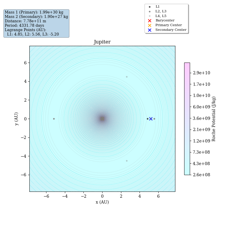
L4, L5 (木星の公転軌道上の60度離れた点)
-
特徴
太陽-木星系のL4およびL5は非常に安定で、多くの小惑星が集まる「トロヤ群小惑星」が存在します。この群は安定性が高く、数百万年スケールで動的に維持されます。 -
関連する小惑星
-
トロヤ群小惑星
- L4(木星の前方60度): 「ギリシャ群」とも呼ばれ、ギリシャ神話に登場する英雄の名前が付けられた小惑星群。
- L5(木星の後方60度): 「トロヤ群」とも呼ばれ、トロイア戦争のトロイア側の登場人物の名前が付けられた小惑星群。
-
代表的な小惑星
- 588 Achilles(L4): トロヤ群小惑星の最初の発見例。
- 624 Hektor(L5): トロヤ群の中で最大級の小惑星。
- その他、小惑星は10,000個以上が確認されており、その多くがこれらのラグランジュ点に集まっています。
-
トロヤ群小惑星
例3: Cygnus X-1

例4: Centaurus X-3

簡単な歴史の紹介
最後に歴史的経緯を確認しておきます。
制限3体問題とロッシュポテンシャルの歴史的背景
制限3体問題とは
制限3体問題は、天体力学の中で重要な研究分野の一つであり、以下の状況を考えます:
- 二つの大質量天体(例:恒星と惑星)が重力相互作用で運動している。
- 三つ目の質量が極めて小さい(近似的に無視できる質量)ため、大質量天体の運動には影響を与えない。
- 三つ目の天体の運動を大質量天体の運動に基づいて解析する。
この問題は、2体問題(天体同士の軌道計算が正確な解を持つ)を拡張し、より複雑な現実世界の系をモデル化するために研究されました。
歴史的背景
1. アイザック・ニュートン (17世紀後半)
ニュートンは「万有引力の法則」と「運動の法則」を確立し、2体問題において正確な解が得られることを示しました。しかし、2体ではない複雑な系では、解析解を得ることが困難であることも認識していました。
2. レオンハルト・オイラー (18世紀中盤)
オイラーは、制限3体問題の特別な解を探求し、二つの大質量天体を結ぶ直線上に存在する3つの点(現在の L1, L2, L3)を発見しました。これらの点では、質量が小さい物体が静止できると示されました。
3. ジョゼフ=ルイ・ラグランジュ (1772年)
ラグランジュは、オイラーの結果を拡張し、二つの天体を頂点とする正三角形の頂点にあたる L4, L5 の存在を理論的に示しました。この発見は、重力と遠心力が均衡する点の数学的特性を深く掘り下げた成果です。
4. エドゥアール・ロッシュ (19世紀中盤)
ロッシュは、ロッシュポテンシャルを用いて制限3体問題を定式化しました。ロッシュは、特に潮汐力やラグランジュ点の安定性の研究を通じて、このポテンシャルが天文学や連星系の動力学の解析において中心的な役割を果たすことを示しました。
ロッシュポテンシャルの重要性
ロッシュポテンシャルは、以下の理由から制限3体問題の解析において重要です:
-
ラグランジュ点の解析
ロッシュポテンシャルの勾配がゼロとなる点を求めることで、質量が小さい天体が力学的に安定する位置を特定できます。 -
潮汐力の解析
ロッシュポテンシャルの等高線を用いると、潮汐力による物質の流れや、天体が潮汐崩壊する閾値を視覚的に解析できます。特にロッシュローブの概念は、連星系における降着円盤形成の重要な指標です。 -
連星系の進化
ロッシュポテンシャルは、ブラックホール連星や中性子星連星といった高エネルギー天文学の系において、物質の移動やエネルギー放出を解析する基盤となります。
制限3体問題の現代的意義
制限3体問題の研究は、天文学や物理学において未だ重要なテーマです。具体的には以下の分野で活用されています:
-
トロヤ群小惑星の解析
L4, L5 に位置する小惑星(トロヤ群)は、太陽と木星の重力によって安定化されています。これはラグランジュの理論の実証例です。 -
惑星形成のモデル
原始惑星系円盤における物質の運動は、制限3体問題の枠組みで理解されます。 -
人工衛星の軌道設計
ラグランジュ点は、人工衛星(例:L1のSOHO衛星、L2のJWST)の配置において利用されています。 -
高エネルギー連星系の降着流の解析
連星系における物質の降着やロッシュローブ越えの動力学解析に制限3体問題が用いられます。
まとめ
制限3体問題とロッシュポテンシャルは、天体力学と天文学の中で長い歴史を持つ課題です。ニュートン、オイラー、ラグランジュ、ロッシュといった研究者の貢献によって、現在の天文学の基礎が築かれました。この理論は、現代の人工衛星や連星系の研究においても中心的な役割を果たしています。