はじめに
恒星の星風(stellar wind)は、恒星表面から流れ出るガスやプラズマの流れで、その速度や密度は恒星の物理的性質を探る上で重要です。本記事では、次のブラックホール連星 Cyg X-1 の星風モデルを基に、Pythonを使ったシミュレーションと可視化を行います。
星風はCAK(Castor, J. I., Abbott, D. C.,Klein, R. I. の頭文字)モデルという有名なモデルがあり、これにより、速度が動径方向に対して変化する状況、つまり dv/dr が 0 ではない場合には、炭素、酸素、窒素など、星の発する紫外線に帯域に多くの吸収バンドを持つ元素は吸収して、ラインフォースで加速し、加速したことでまた別の周波数の光を吸収することができるようになり、トータルでは脱出速度まで星風加速が起こる可能性が示され、いまでは星風モデルの標準的なモデルになっています。
Cyg X-1 の星風モデル (Gies, D. R., Bolton, C. T. 1986)
Cyg X-1 の星風モデルについては、
の式(1),(2,(3)および Table1 を用いた計算が簡易的なモデルになります。下記ではその計算方法を可視化について紹介します。
星風モデルの数式
星風の速度 $ v_{\text{wind}} $ と密度 $ \rho_{\text{wind}} $ は次のように表現されます。
星風の速度
v_{\text{wind}} = v_{\infty}(\theta) \left[ 1 - \frac{r^*(\theta)}{r} \right]^{a(\theta)}
- $ v_{\infty}(\theta) $: 終端速度(角度 $ \theta $ の関数)
- $ r^*(\theta) $: 星風開始半径(角度 $ \theta $ の関数)
- $ a(\theta) $: パラメータ(角度 $ \theta $ の関数)
星風の密度
\rho_{\text{wind}} = \left[ \frac{r^*(\theta)}{r} \right]^2 \frac{\rho_0(\theta)}{\left\{1 - \left[\frac{r^*(\theta)}{r}\right]\right\}^{a(\theta)}}
- $ \rho_0(\theta) $: 星風密度の基準値(角度 $ \theta $ の関数)
パラメータの補間
角度 $ \theta $ が $ 0^\circ $ から $ 20^\circ $ の間では、次のルールに基づき補間を行います:
X(r, \theta) = X(r, 0^\circ) + \left[ X(r, 20^\circ) - X(r, 0^\circ) \right] \left( \frac{\theta}{20^\circ} \right)^2
つまり、 $ \theta $ に対して直線的に補間し、連続的な変化を再現します。
星風モデルのパラメータ
次の表に、モデルの角度ごとのパラメータを示します。
d は連星間距離(ブラックホールと星)として、上の論文では、星の半径($\theta=0$; ブラックホール方向)が 0.5 d と 0.4 d の2つのパターンについて考えます。
| 星の半径 (d) | $ \theta $ ($ ^\circ $) | $ r^* $ ($ 10^{12} $ cm) | $ a $ | $ v_\infty $ (km/s) | $ \rho_0 $ ($ 10^{-14} $ g/cm$^3$) |
|---|---|---|---|---|---|
| 0.5 | 0 | 1.496 | 1.60 | 2540 | 6.17 |
| 20 | 1.387 | 1.05 | 1580 | 3.72 | |
| 0.4 | 0 | 1.197 | 1.16 | 2030 | 4.01 |
| 20 | 1.157 | 0.96 | 1650 | 4.61 |
Pythonによる計算と可視化
プログラムの全コード
以下のPythonコードを用いて、速度と密度を計算し、可視化を行います。
#!/usr/bin/env python

import numpy as np
import matplotlib.pyplot as plt

# Set font properties for plots
plt.rcParams['font.family'] = 'serif'

# Define constants
INCLINATION = 30  # Viewing inclination in degrees

# Stellar wind parameters for different models (stellar radius scaling factor)
parameters = {
    0.5: {
        0: {"r_star": 1.496e12, "a": 1.60, "v_inf": 2540, "rho_0": 6.17e-14},
        20: {"r_star": 1.387e12, "a": 1.05, "v_inf": 1580, "rho_0": 3.72e-14},
    },
    0.4: {
        0: {"r_star": 1.197e12, "a": 1.16, "v_inf": 2030, "rho_0": 4.01e-14},
        20: {"r_star": 1.157e12, "a": 0.96, "v_inf": 1650, "rho_0": 4.61e-14},
    },
}

def interpolate(value_0, value_20, theta):
    """Interpolates parameter values for a given angle θ between 0° and 20°."""
    return value_0 + (value_20 - value_0) * (theta / 20) ** 2

def v_wind(r, theta, stellar_radius):
    """Calculates the wind velocity at a given radius and angle."""
    params = parameters[stellar_radius]
    r_star_theta = interpolate(params[0]["r_star"], params[20]["r_star"], theta)
    a_theta = interpolate(params[0]["a"], params[20]["a"], theta)
    v_inf_theta = interpolate(params[0]["v_inf"], params[20]["v_inf"], theta)

    if 1 - r_star_theta / r > 0:
        velecoty_wind = v_inf_theta * (1 - r_star_theta / r) ** a_theta
    else:
        velecoty_wind = 0
    return velecoty_wind

def rho_wind(r, theta, stellar_radius):
    """Calculates the wind density at a given radius and angle."""
    params = parameters[stellar_radius]
    r_star_theta = interpolate(params[0]["r_star"], params[20]["r_star"], theta)
    rho_0_theta = interpolate(params[0]["rho_0"], params[20]["rho_0"], theta)
    a_theta = interpolate(params[0]["a"], params[20]["a"], theta)
    numerator = (r_star_theta / r) ** 2 * rho_0_theta
#    print(f"r_star_theta / r = {r_star_theta} / {r}, a_theta = {a_theta}")
    if 1 - (r_star_theta / r) > 0:
        denominator = (1 - (r_star_theta / r)) ** a_theta
        adensity_wind = numerator / denominator
    else:
        adensity_wind = 0
    return adensity_wind

def plot_v_rho(stellar_radius):
    """Generates and saves plots for wind velocity, density profiles, and projected velocities."""
    solar_radius = 6.96e10  # Solar radius in cm
    stellar_radius_in_solar = 22  # Stellar radius in units of solar radius
    r_values = np.linspace(solar_radius, 50 * solar_radius, 500)
    theta_values = [0, 5, 10, 15, 20]

    # Plot wind velocity and density profiles
    fig, axes = plt.subplots(1, 2, figsize=(14, 6))
    fig.suptitle(f"Stellar Radius = {stellar_radius} binary separation (d)"  + f"{stellar_radius_in_solar}  " + r"$R_{star}$=" + f"{stellar_radius_in_solar}" + r"$R_{\odot}$", fontsize=12)

    # Wind velocity profiles
    ax1 = axes[0]
    ax2 = ax1.secondary_xaxis('top', functions=(lambda x: x / stellar_radius_in_solar,
                                                lambda x: x * stellar_radius_in_solar))
    ax2.set_xlabel(r"$R$ [$R_{star}$]")
    for theta in theta_values:
        v_values = [v_wind(r, theta, stellar_radius) for r in r_values]
        line, = ax1.plot(r_values / solar_radius, v_values, label=f"Theta = {theta} deg")

        v_inf_theta = interpolate(
            parameters[stellar_radius][0]["v_inf"],
            parameters[stellar_radius][20]["v_inf"],
            theta,
        )
        ax1.axhline(y=v_inf_theta, color=line.get_color(), linestyle="--", label=f"v_inf ({theta} deg)")

    ax1.set_xlabel(r"$R$ [$R_{\odot}$]")
    ax1.set_ylabel(r"$v_{wind}$ [km/s]")
    ax1.legend()
    ax1.grid(alpha=0.5)

    # Wind density profiles
    ax3 = axes[1]
    ax4 = ax3.secondary_xaxis('top', functions=(lambda x: x / stellar_radius_in_solar,
                                                lambda x: x * stellar_radius_in_solar))
    ax4.set_xlabel(r"$R$ [$R_{star}$]")

    m_H = 1.67e-24  # Hydrogen atom mass [g]
    mu = 1  # Mean molecular weight
    ax5 = ax3.secondary_yaxis('right', functions=(lambda rho: rho / (mu * m_H),
                                                  lambda n: n * (mu * m_H)))
    ax5.set_ylabel(r"$n_{wind}$ [cm$^{-3}$]")

    for theta in theta_values:
        rho_values = [rho_wind(r, theta, stellar_radius) for r in r_values]
        ax3.plot(r_values / solar_radius, rho_values, label=f"Theta = {theta} deg")
    ax3.set_xlabel(r"$R$ [$R_{\odot}$]")
    ax3.set_ylabel(r"$\rho_{wind}$ [g/cm³]")
    ax3.set_yscale("log")
    ax3.legend()
    ax3.grid()

    plt.tight_layout()
    plt.savefig(f"stellar_profile_{stellar_radius}.png", bbox_inches='tight')
    plt.show()

    # Plot projected wind velocities
    r_values_forproj = np.linspace(solar_radius * 25, 50 * solar_radius, 5)
    fig, axes = plt.subplots(len(theta_values), 1, figsize=(10, 8), sharex=True)
    fig.subplots_adjust(right=0.8)
    fig.suptitle(f"Projected Velocities: Stellar Radius = {stellar_radius} binary separation (d) \n" + f"inclination = {INCLINATION} (deg)   " + r"$R_{star}$=" + f"{stellar_radius_in_solar}" + r"$R_{\odot}$", fontsize=12)

    for i, theta in enumerate(theta_values):
        v_values = [v_wind(r, theta, stellar_radius) for r in r_values_forproj]
        for v, r in zip(v_values, r_values_forproj):
            phase = np.linspace(0, 4 * np.pi, 100)
            view_angle = -np.cos(phase) * np.deg2rad(INCLINATION)
            v_proj = v * np.sin(np.deg2rad(theta) - view_angle)
            axes[i].plot(phase / (2 * np.pi), v_proj, label=f"$\\theta$={theta} deg, $R={r / solar_radius:.1f}$ Rsun")
            axes[i].set_ylabel(r"$v_{proj}$ [km/s]")
            axes[i].legend(loc='center left', bbox_to_anchor=(1, 0.5), fontsize=8)
            axes[i].grid(alpha=0.3)
            axes[i].set_ylim(-1000,1000)

    axes[-1].set_xlabel("Orbital Phase")
    plt.tight_layout()
    plt.savefig(f"stellar_profile_{stellar_radius}_proj.png", bbox_inches='tight')
    plt.show()

# Main execution
if __name__ == "__main__":
    for stellar_radius in [0.5, 0.4]: # stallar radius in unit of binary separation
        plot_v_rho(stellar_radius)
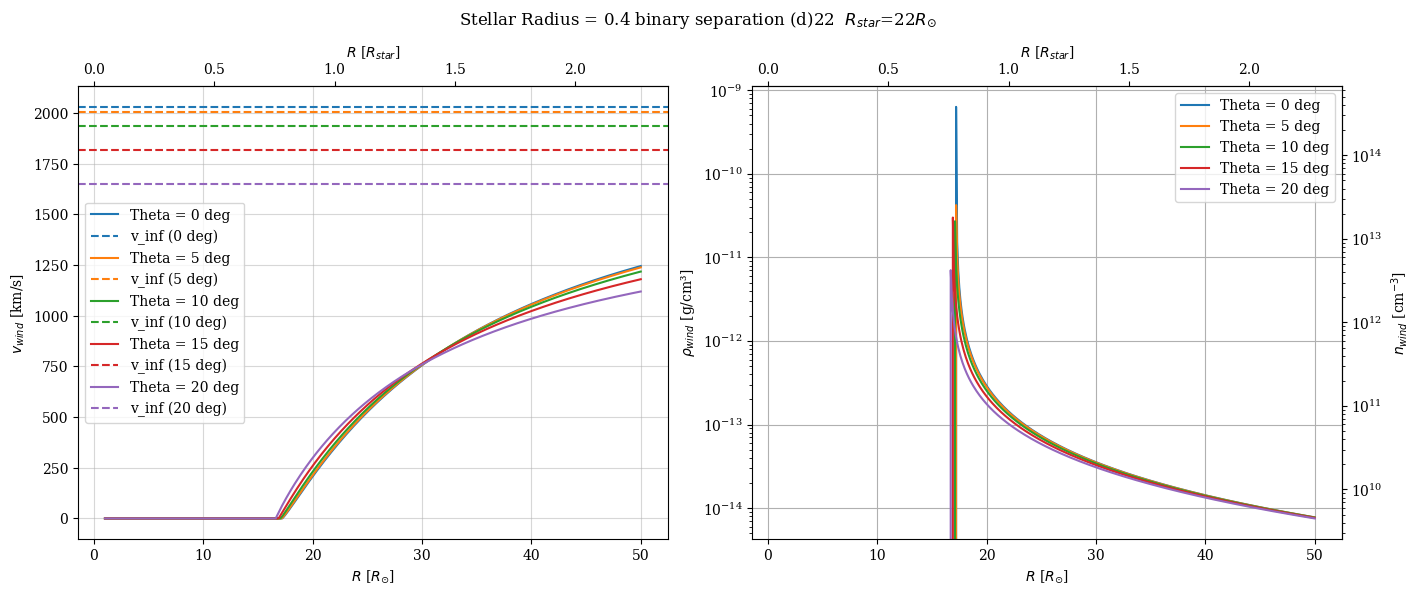
結果のグラフと解釈
密度と速度プロファイル
- 星の半径が 0.4 d の場合
- 星の半径が 0.5 d の場合

-
速度プロット:
半径 $ r $ が増加すると、速度 $ v_{\text{wind}} $ は終端速度に近づきます。角度 $ \theta $ が増加するほど、終端速度は減少します。 -
密度プロット:
密度 $ \rho_{\text{wind}} $ は $ r $ が増加するほど減少します。
projected な wind 速度
単純に、計算すると、、だめですね。gies et al. を拡張しないと計算が絶対にできないはず。。
補足
手前味噌ですが、昔の回転入りの計算などと比べても、オーダーは大間違いはしてないと思われる。
まとめ
本記事では、星風モデルの基礎式を用いて、Pythonで計算と可視化を行いました。このコードを応用することで、ブラックホール連星 Cyg X-1 の基礎的な挙動を考えるキッカケになれば幸いです。