本シリーズのモチベーション
データ解析のための統計モデリング入門の内容について理解を深めることを目的に、本書で例示されていた統計モデリング・データ解析に関する処理をPythonでコーディングします(本書ではRでコーディングされていました)。
注:記事は簡潔に書こうと思いますので、本書をご購入・ご一読の上でないと、理解が難しいです。
2章(本ページ):データ解析のための統計モデリング入門 2章 Pythonによるコーディング
3章:データ解析のための統計モデリング入門 3章 Pythonによるコーディング
6章:データ解析のための統計モデリング入門 6章 Pythonによるコーディング
7章:データ解析のための統計モデリング入門 7章 Pythonによるコーディング
2章を読むモチベーション
統計モデルの基本部品である確率分布(ポアソン分布を例にとる)により、データのばらつきが表現できることを理解する。モデルのパラメータを推定する方法である最尤推定への理解を深める。
ポアソン分布に従うデータの観察
データの生成(サンプリング)
データの生成(サンプリング)を行います。
import numpy as np
import matplotlib.pyplot as plt
from scipy.stats import poisson, norm, binom
from scipy.optimize import minimize_scala

def generate_poisson_data(lam, size):
  """
  ポアソン分布に従うデータを生成する関数

  Args:
    lam: ポアソン分布の平均
    size: 生成するデータの数

  Returns:
    ポアソン分布に従うデータのリスト
  """
  return np.random.poisson(lam, size)

data = generate_poisson_data(lam=3.5, size=50)
print(data)
[6 2 2 2 3 4 2 4 6 2 3 2 4 7 2 1 3 5 3 2 4 8 2 4 1
2 3 9 3 2 2 3 2 7 2 6 2 5 2 4 3 6 6 2 0 1 2 6 8 3]
生成(サンプリング)したデータの要約
生成(サンプリング)したデータの要約を行います。
def summarize_integer_data(data):
  """
  整数値データの最小値、第一四分位数、中央値、平均、第三四分位数、最大値を出す関数

  Args:
    data: 整数値データのリスト

  Returns:
    最小値、第一四分位数、中央値、平均、第三四分位数、最大値のタプル
  """
  min_value = np.min(data)
  q1 = np.percentile(data, 25)
  median = np.median(data)
  mean = np.mean(data)
  q3 = np.percentile(data, 75)
  max_value = np.max(data)
  return min_value, q1, median, mean, q3, max_value

min_value, q1, median, mean, q3, max_value = summarize_integer_data(data)

print("最小値:", min_value)
print("第一四分位数:", q1)
print("中央値:", median)
print("平均:", mean)
print("第三四分位数:", q3)
print("最大値:", max_value)
最小値: 0
第一四分位数: 2.0
中央値: 3.0
平均: 3.5
第三四分位数: 4.75
最大値: 9
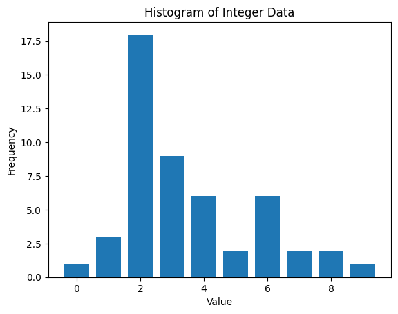
生成(サンプリング)したデータの図示と標本統計量の計算
生成(サンプリング)したデータの図示を行います。
def plot_integer_histogram(data):
  """
  整数値データのヒストグラムを描く関数

  Args:
    data: 整数値データのリスト
  """
  plt.hist(data, bins=np.arange(np.min(data), np.max(data) + 2) - 0.5, rwidth=0.8)
  plt.xlabel('Value')
  plt.ylabel('Frequency')
  plt.title('Histogram of Integer Data')
  plt.show()

plot_integer_histogram(data)
データの分散・標準偏差を求めます。
def calculate_variance_std(data):
  """
  整数値配列データの分散、標準偏差を求める関数

  Args:
    data: 整数値データのリスト

  Returns:
    分散、標準偏差のタプル
  """
  variance = np.var(data)
  std = np.std(data)
  return variance, std

variance, std = calculate_variance_std(data)

print("分散:", variance)
print("標準偏差:", std)
分散: 4.25
標準偏差: 2.0615528128088303
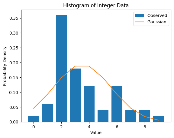
種々の有名な分布の理論値とサンプリングしたデータの比較
種々の有名な分布の理論値とサンプリングしたデータを重ねて比較します。
def plot_histogram_with_theoretical_dist(data, dist_name=None, **kwargs):
  """
  整数値データのヒストグラムを描き、指定された分布の理論的な分布を重ねて表示する関数

  Args:
    data: 整数値データのリスト
    dist_name: 分布名 ('poisson', 'gaussian', 'binomial')
    **kwargs: 分布のパラメータ (例: lam=3.56 for Poisson, mu=0, sigma=1 for Gaussian, n=10, p=0.5 for Binomial)
  """
  plt.hist(data, bins=np.arange(np.min(data), np.max(data) + 2) - 0.5, rwidth=0.8, density=True, label='Observed')
  plt.xlabel('Value')
  plt.ylabel('Probability Density')
  plt.title('Histogram of Integer Data')

  if dist_name is not None:
    x = np.arange(np.min(data), np.max(data) + 1)
    if dist_name == 'poisson':
      lam = kwargs.get('lam')
      if lam is None:
        raise ValueError("Poisson distribution requires 'lam' parameter.")
      plt.plot(x, poisson.pmf(x, lam), label='Poisson')
    elif dist_name == 'gaussian':
      mu = kwargs.get('mu', 0)
      sigma = kwargs.get('sigma', 1)
      plt.plot(x, norm.pdf(x, mu, sigma), label='Gaussian')
    elif dist_name == 'binomial':
      n = kwargs.get('n')
      p = kwargs.get('p')
      if n is None or p is None:
        raise ValueError("Binomial distribution requires 'n' and 'p' parameters.")
      plt.plot(x, binom.pmf(x, n, p), label='Binomial')
    else:
      raise ValueError("Invalid distribution name. Choose from 'poisson', 'gaussian', or 'binomial'.")
    plt.legend()

  plt.show()

# 例:ポアソン分布を重ねて表示
plot_histogram_with_theoretical_dist(data, dist_name='poisson', lam=3.56)

# 例:ガウス分布を重ねて表示
plot_histogram_with_theoretical_dist(data, dist_name='gaussian', mu=np.mean(data), sigma=np.std(data))

# 例:二項分布を重ねて表示
plot_histogram_with_theoretical_dist(data, dist_name='binomial', n=10, p=0.3)


最尤推定(ポアソン分布を仮定して)
def calculate_log_likelihood(data, lam):
  """
  実測値から対数尤度を計算する関数

  Args:
    data: 実測値のリスト
    lam: ポアソン分布のパラメータ

  Returns:
    対数尤度
  """
  log_likelihood = np.sum(poisson.logpmf(data, lam))
  return log_likelihood

def calculate_max_log_likelihood(data):
  """
  実測値から最大対数尤度を計算し、最大対数尤度とその時のパラメータを返す関数

  Args:
    data: 実測値のリスト

  Returns:
    最大対数尤度と、その時のパラメータのタプル
  """
  def negative_log_likelihood(lam):
    return -calculate_log_likelihood(data, lam)

  res = minimize_scalar(negative_log_likelihood, bounds=(0, 100), method='bounded')
  max_log_likelihood = -res.fun
  optimal_param = res.x
  return max_log_likelihood, optimal_param

# 最大対数尤度と最適なパラメータを計算
max_log_likelihood, optimal_param = calculate_max_log_likelihood(data)

print("最大対数尤度:", max_log_likelihood)
print("最適なパラメータ:", optimal_param)
最大対数尤度: -103.54913473386503
最適なパラメータ: 3.4999989598683987