はじめに
KaggleのSpotifyデータセットを使用して色々と分析してみました。
他の方のコードを参考に色々といじってみたので
アウトプット用として始めて記事を投稿します。
使用環境
MacOS
Python 3.8.10
JupyterLab 3.0.14
今回使用したデータ
Spotify Dataset 1922-2021
100年分のデータがまとまっており、曲数も約60万件も含まれているデータです。
インポート
まずは必要なライブラリのインポート。
import numpy as np
import pandas as pd
import matplotlib.pyplot as plt
from matplotlib.font_manager import FontProperties
%matplotlib inline
import seaborn as sns

from tqdm import tqdm
import time
import datetime
曲のデータをダウンロード
データはtracks.csvを使用します。
# 曲名詳細
tracks = pd.read_csv("tracks.csv")
tracks.head(3)
| id | name | popularity | duration_ms | explicit | artists | id_artists | release_date | danceability | energy | key | loudness | mode | speechiness | acousticness | instrumentalness | liveness | valence | tempo | time_signature | |
|---|---|---|---|---|---|---|---|---|---|---|---|---|---|---|---|---|---|---|---|---|
| 0 | 35iwgR4jXetI318WEWsa1Q | Carve | 6 | 126903 | 0 | ['Uli'] | ['45tIt06XoI0Iio4LBEVpls'] | 1922-02-22 | 0.645 | 0.445 | 0 | -13.338 | 1 | 0.4510 | 0.674 | 0.7440 | 0.151 | 0.127 | 104.851 | 3 |
| 1 | 021ht4sdgPcrDgSk7JTbKY | Capítulo 2.16 - Banquero Anarquista | 0 | 98200 | 0 | ['Fernando Pessoa'] | ['14jtPCOoNZwquk5wd9DxrY'] | 1922-06-01 | 0.695 | 0.263 | 0 | -22.136 | 1 | 0.9570 | 0.797 | 0.0000 | 0.148 | 0.655 | 102.009 | 1 |
| 2 | 07A5yehtSnoedViJAZkNnc | Vivo para Quererte - Remasterizado | 0 | 181640 | 0 | ['Ignacio Corsini'] | ['5LiOoJbxVSAMkBS2fUm3X2'] | 1922-03-21 | 0.434 | 0.177 | 1 | -21.180 | 1 | 0.0512 | 0.994 | 0.0218 | 0.212 | 0.457 | 130.418 | 5 |
| name | album | artists | release_date | length | popularity | danceability |
acousticness | energy | instrumentalness | mode | liveness |
loudness | speechiness | valence |
tempo | time_signature | ||||
| 曲名 | アルバム名 | アーティスト名 | リリース日 | 曲の長さ | 人気度 | ダンス度 0.0-1.0 |
アコースティック度 0.0-1.0 |
エネルギー 0.0-1.0 | インスト感 0.0-1.0 |
曲調を示す | ライブさ 0.0-1.0 |
音の大きさ -60 〜 0 db | スピーチ度 |
曲のポジティブ度 |
曲のテンポ | 拍子 | ||||
| 曲ごとに色々なパラメーターが付与されています。 | ||||||||||||||||||||
| 詳しくは、Spotifyドキュメントに書いてあります。 | ||||||||||||||||||||
| https://developer.spotify.com/documentation/web-api/reference/#objects-index |
曲のデータ分析を実践してみる
データ整形
release_dateを年と月単位にして, 必要のないカラムを削除
tracks["release_date"] = pd.to_datetime(tracks["release_date"])
tracks["release_year"] = tracks["release_date"].dt.year
tracks["release_month"] = tracks["release_date"].dt.month
cols_to_drop = ["id","id_artists","release_date"]
tracks.drop(columns=cols_to_drop,inplace=True)
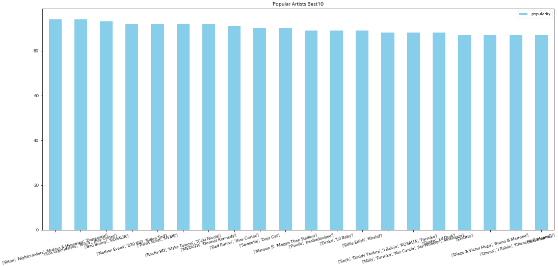
人気アーティストTop20
tracks.groupby("artists")["popularity"].mean().sort_values(ascending = False).to_frame()[: 20].plot(kind="bar",figsize=(18,8),color="skyblue",rot=30,title="Popular Artists Best10")
特徴量の相関関係を可視化
tracks_df.drop(["explicit","key","explicit","mode","time_signature","release_month"],axis=1,inplace=True)
# corrメソッド = 各列の間の相関係数が算出される
corr = tracks_df.corr()
plt.figure(figsize=(14,8))
sns.heatmap(corr,annot=True,fmt='.2f',cmap='RdBu_r')
plt.savefig("corr_image")
plt.show()
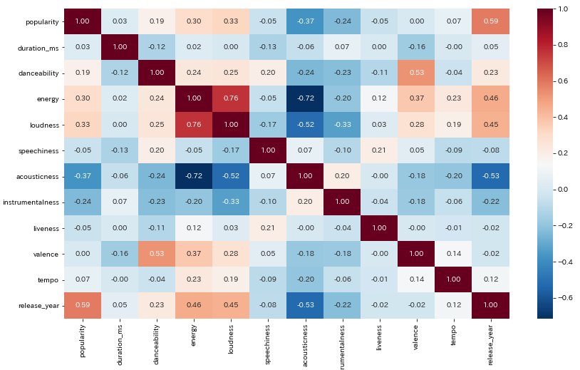
この相関図から考えられること
- yearとpopularity 年数を重ねるごとに人気度が高い(最近の曲の方が評価する人が多い)
- enegyとloudness 音が大きいジャンルはfast, loud, noisyである可能性が高い
- yearとloundness & enegy ここ20年あたりのロックやHIPHOPの影響であると思う
- popularityとloundness & enegy 上がる曲が人気(必然的)
- acousticnessとloundness & enegy 落ち着いているためまあ分かる
- acousticnessとyear 年々アコースティックの曲が減っている?
- loundnessとinstrumentalness 負相関な理由は疑問(音の大きさは楽器に影響していない?)
特徴量の年推移を比較した折線グラフ
features_to_plot = ['energy', 'acousticness','instrumentalness', 'speechiness',"danceability"]
plt.figure(figsize=(14,8))
before = time.time()
for i in tqdm(features_to_plot):
    sns.lineplot(x="release_year",y=i,data=tracks)

plt.legend(features_to_plot)
plt.ylabel("value")
after = time.time()
print("it took {}".format(after - before))
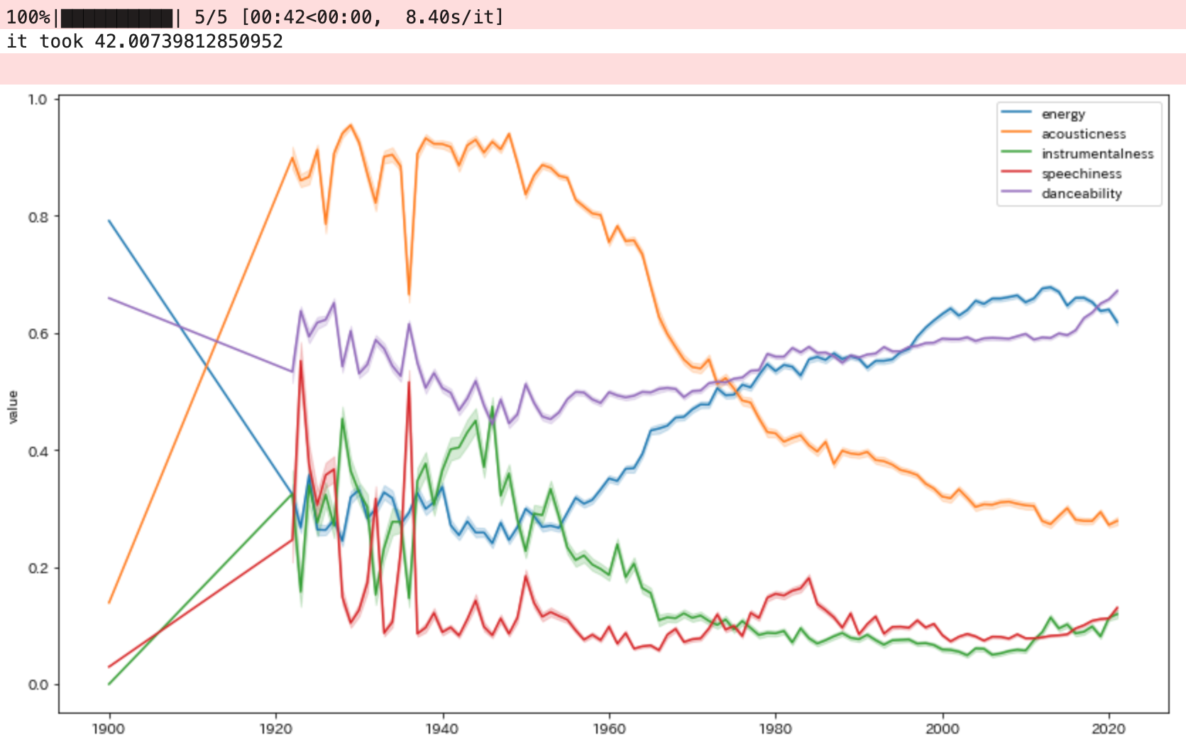
・1945年の終戦前ではジャズやブルース、ゴスペルの流行にともない
スピーチ度やアコースティック度、インスト感などが高い傾向があります。
・逆に1960年代のイギリスロックシーンなどが流行すると
曲の速さ,大きさ,うるささが高くなっています。
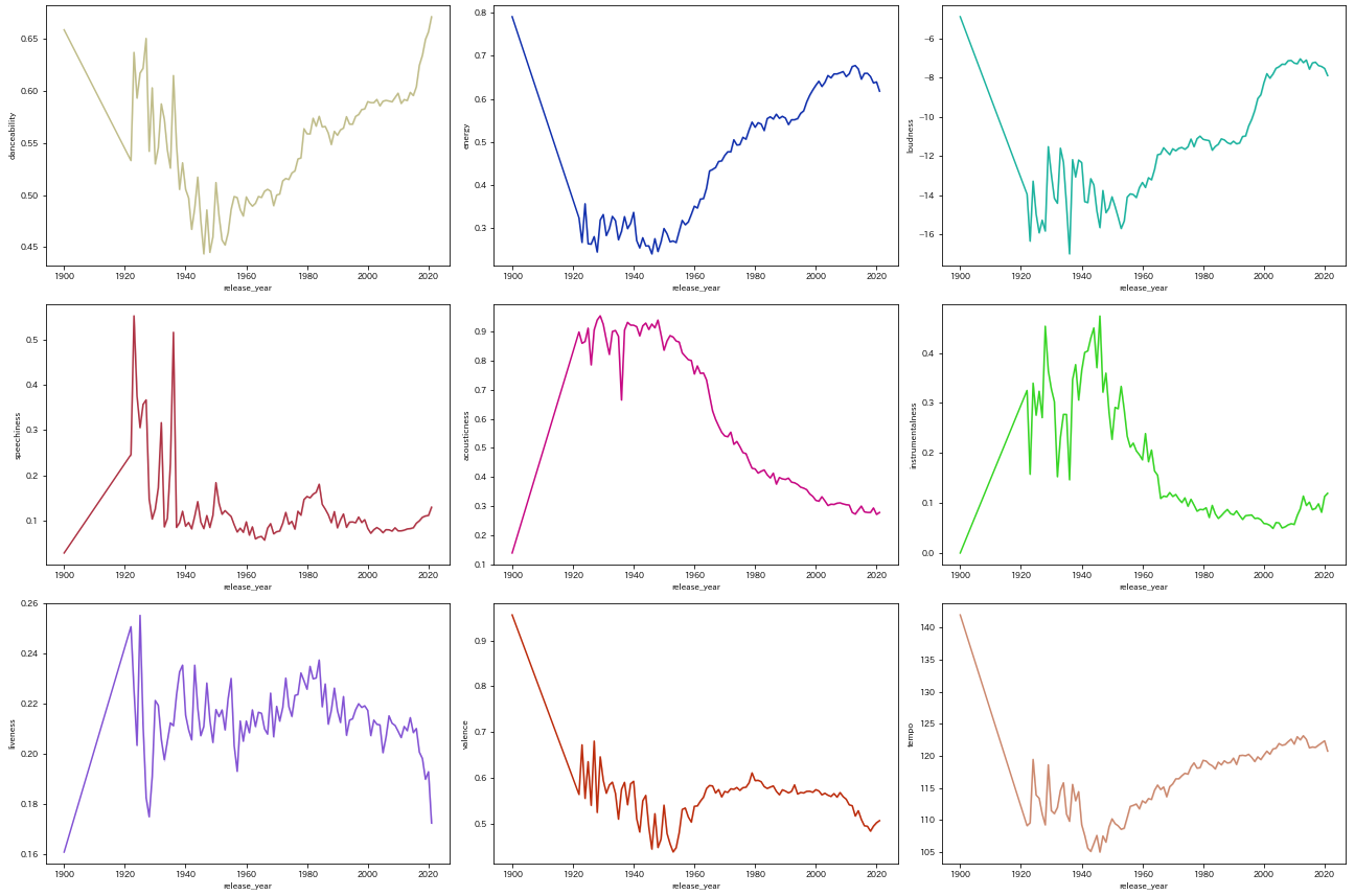
各特徴量の年推移を折線グラフでまとめてみた
features_to_plot = [['danceability','energy','loudness'],['speechiness','acousticness','instrumentalness'],['liveness','valence','tempo']]
fig,axes = plt.subplots(3,3,figsize=(18,12))
before = time.time()
for i in tqdm(range(3)):
    for l in range(3):
        color = np.random.rand(3,)
        sns.lineplot(x="release_year",y=features_to_plot[i][l],data=tracks,ax=axes[i][l],color=color,ci=False)
plt.tight_layout()
plt.show()
after = time.time()
print("it took {}".format(after - before))
各特徴別のartistランキング Top5
features_to_plot = [['danceability','energy','loudness'],['speechiness','acousticness','instrumentalness'],['liveness','valence','tempo']]
fig,axes = plt.subplots(3,3,figsize=(25,20))
before = time.time()
for i in tqdm(range(3)):
    for l in range(3):
        color = np.random.rand(3,)
        tracks.groupby("artists")[features_to_plot[i][l]].mean().sort_values(ascending = False).to_frame()[: 5].plot(kind="bar",ax=axes[i][l],color=color,rot=20,title="Top5 artists for {}".format(features_to_plot[i][l]))

plt.show()
plt.tight_layout()
after = time.time()
print("it took {}".format(after - before))
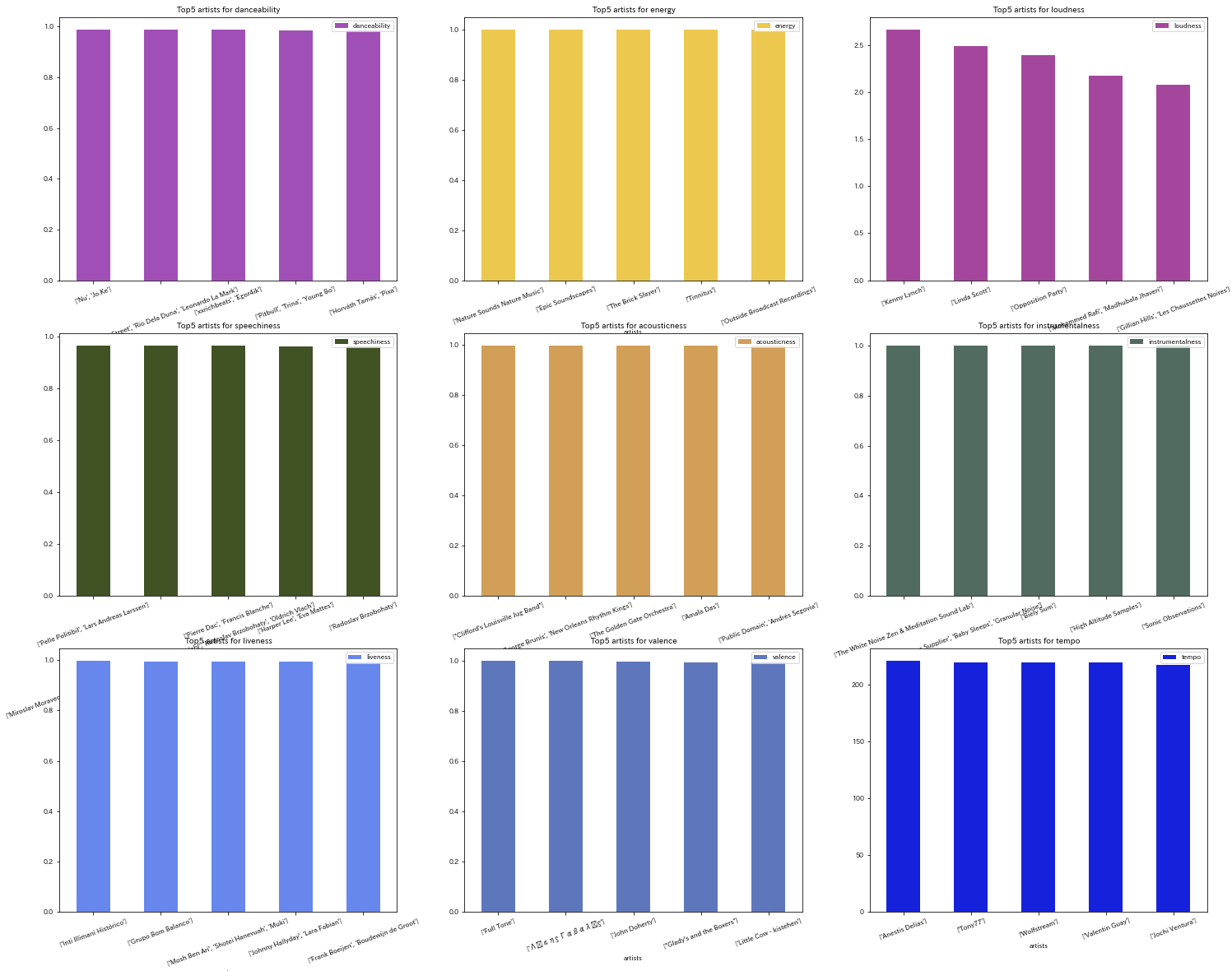
アーティスト名が長くて収まりませんでした。見にくくてすみません。
曲のジャンルを分析してみる
今度は曲のジャンルごとによる分析をしていきたいと思います。
データはdata_by_genres_o.csvを使用します。
ジャンルのデータをダウンロード
# ジャンル詳細
genres_detail = pd.read_csv("data_by_genres_o.csv")
genres_detail.head(3)
| mode | genres | acousticness | danceability | duration_ms | energy | instrumentalness | liveness | loudness | speechiness | tempo | valence | popularity | key | |
|---|---|---|---|---|---|---|---|---|---|---|---|---|---|---|
| 0 | 1 | 21st century classical | 0.979333 | 0.162883 | 1.602977e+05 | 0.071317 | 0.606834 | 0.3616 | -31.514333 | 0.040567 | 75.336500 | 0.103783 | 27.833333 | 6 |
| 1 | 1 | 432hz | 0.494780 | 0.299333 | 1.048887e+06 | 0.450678 | 0.477762 | 0.1310 | -16.854000 | 0.076817 | 120.285667 | 0.221750 | 52.500000 | 5 |
| 2 | 1 | 8-bit | 0.762000 | 0.712000 | 1.151770e+05 | 0.818000 | 0.876000 | 0.1260 | -9.180000 | 0.047000 | 133.444000 | 0.975000 | 48.000000 | 7 |
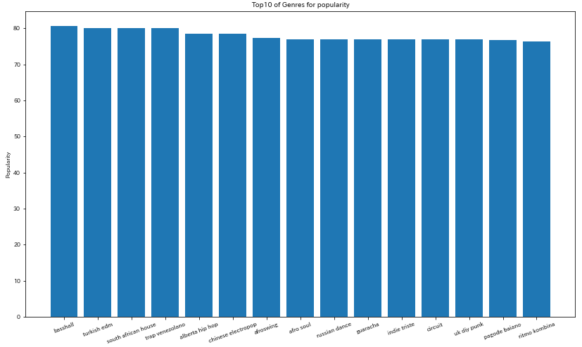
人気ジャンルTop15
HIPHOPやROCKなどの大元のジャンルからの派生ジャンルが多いため
聞いたことのないコアなジャンルばかりですね(・ ・;)
top_10_genres = genres_detail.sort_values(by="popularity",ascending= False).head(15)
plt.figure(figsize=(14,8))
plt.bar(top_10_genres["genres"],top_10_genres["popularity"])
plt.xlabel('Genre')
plt.ylabel('Popularity')
plt.xticks(rotation=20)
plt.title('Top10 of Genres for popularity')
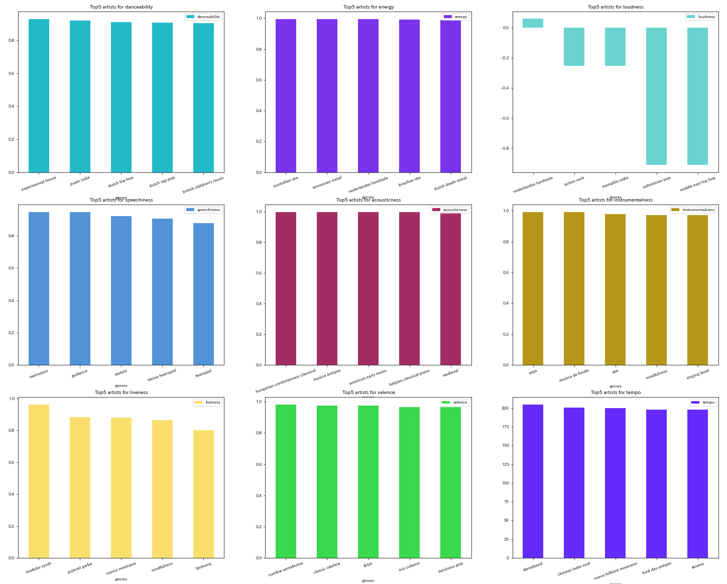
各特徴別のgenresランキング Top5
例のごとく各特徴量ごとの人気ジャンルを順位付けしていきます。
features_to_plot = [['danceability','energy','loudness'],['speechiness','acousticness','instrumentalness'],['liveness','valence','tempo']]
fig,axes = plt.subplots(3,3,figsize=(25,20))
before = time.time()
for i in tqdm(range(3)):
    for l in range(3):
        color = np.random.rand(3,)
        genres_detail.groupby("genres")[features_to_plot[i][l]].mean().sort_values(ascending = False).to_frame()[: 5].plot(kind="bar",ax=axes[i][l],color=color,rot=20,title="Top5 artists for {}".format(features_to_plot[i][l]))

plt.show()
plt.tight_layout()
after = time.time()
print("it took {}".format(after - before))
多く作曲されている主要ジャンルを分析
派生ジャンルとしてとても細かいジャンルまであるので
ROCKやHIPHOPといった主要なジャンルとして分けたいと思います。
ジャンルのみリスト化
main_name_genres = genres_detail["genres"].to_list()
main_name_genres[:5]
//['21st century classical', '432hz', '8-bit', '[]', 'a cappella']
ワードごとに分割
'21st century classical'が21st, century, classicalと3分割されました
main_name_genres = " ".join(genres_detail["genres"].to_list()).split()
main_name_genres[:5]
//['21st', 'century', 'classical', '432hz', '8-bit']
ワードの出現回数を取得
collectionsモジュールを使用してそれぞれのワードの出現回数を
collections.Counter型(タプル型)として取り出しリスト化する
import collections

genres_tuple = collections.Counter(main_name_genres)
genres_list = list(genres_tuple.items())
genres_list[:5]
//[('21st', 2), ('century', 2), ('classical', 106), ('432hz', 1), ('8-bit', 1)]
データフレーム化
参考にしたサイトです
https://www.delftstack.com/ja/howto/python-pandas/pandas-create-dataframe-from-list/
main_genres = pd.DataFrame(genres_list, columns = ['genres','count'])
main_genres.sort_values('count',ascending=False,inplace=True)
main_genres.reset_index(drop=True).head()
| genres | count | |
|---|---|---|
| 0 | pop | 240 |
| 1 | indie | 237 |
| 2 | rock | 183 |
| 3 | metal | 132 |
| 4 | classical | 106 |
主要ジャンル出現回数を可視化
df = main_genres.head(25)
plt.figure(figsize=(10,6))
sns.barplot(x='count' , y ='genres', data=df)
plt.title('主要ジャンル出現回数ランキング')
plt.ylabel('ジャンル名')
plt.xlabel('出現回数')
plt.show
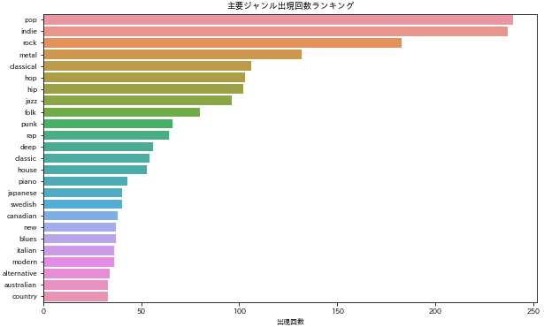
pop, indie, rock, metal, classicalという結果になりました。日本の歌は割と多いみたいです。
上位4つの主要ジャンルから人気派生ジャンルを検証
特に作曲回数の多いpop, indie, rock, metalの人気派生ジャンルを7つ順位付けしました。
参考にしたサイトです https://note.nkmk.me/python-pandas-str-contains-match/
# https://note.nkmk.me/python-pandas-str-contains-match/
pop_df = genres_detail[genres_detail["genres"].str.contains("pop")].sort_values("popularity",ascending=False).head(7)
indie_df = genres_detail[genres_detail["genres"].str.contains("indie")].sort_values("popularity",ascending=False).head(7)
rock_df = genres_detail[genres_detail["genres"].str.contains("rock")].sort_values("popularity",ascending=False).head(7)
metal_df = genres_detail[genres_detail["genres"].str.contains("metal")].sort_values("popularity",ascending=False).head(7)

fig, axes = plt.subplots(2,2,figsize=(16,10))
axes[0,0].barh(width=pop_df['popularity'],y=pop_df['genres'],color="blue")
axes[0,1].barh(width=indie_df['popularity'],y=indie_df['genres'],color="green")
axes[1,0].barh(width=rock_df['popularity'],y=rock_df['genres'],color="orange")
axes[1,1].barh(width=metal_df['popularity'],y=metal_df['genres'],color="red")

fig.tight_layout(pad=1)
fig.show()
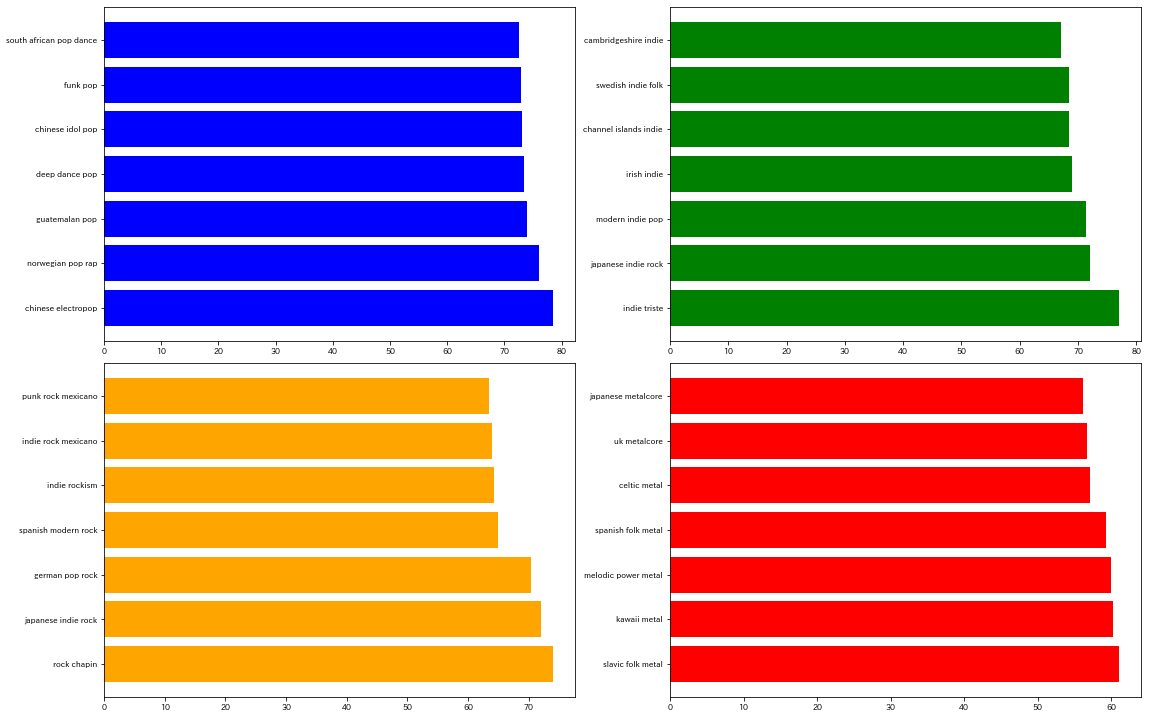
やはり日本のジャンルは人気が高いみたいです。
個人的にkawaii metalがとても気になります(BABYMETAlLみたいな感じですかね?)
まとめ
データ分析初心者としてデータ分析に必要なライブラリを使ってみて
知らない文法にも触れれてよかったです。
予想とは違った結果が多く、データ数も多い面白いデータセットだと思います。
機械学習に何か落とし込めないか模索していきます。