Overview
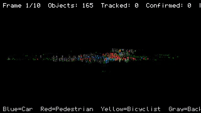
I built a full perception pipeline on 128-beam infrastructure-mounted LiDAR data — ground removal, BEV clustering, Random Forest classification, and Kalman filter multi-object tracking. All classical methods, no deep learning for detection.
This post shares the key engineering lessons — what broke, why, and how I fixed it. The full code and detailed reports are on GitHub:
Repository: https://github.com/bonsai89/lidar-perception-pipeline
The Pipeline
Raw LiDAR (184k points, 128 beams)
    → Ground Removal (RANSAC calibration + polar grid)
    → BEV Clustering (connected components)
    → Classification (Random Forest, 23 geometric features)
    → Multi-Object Tracking (Kalman filter + Hungarian assignment)
    → Classified objects with persistent IDs
Key Lessons
1. Ground Removal: 6 iterations to get right
The sensor is infrastructure-mounted (fixed on a pole, tilted down). I went through 6 approaches:
| Iteration | Method | Why it failed |
|---|---|---|
| 1 | Per-frame RANSAC on full scene | Locked onto bus roof, not road. 6-7s per frame |
| 2 | Calibrate once + flat z-threshold | Missed ground at range where road slopes |
| 3 | Cartesian grid + local percentile | Bus underside corrupted ground estimate in cells below bus |
| 4 | Multi-frame accumulation | Only 1-5% cell coverage across frames |
| 5 | Plane equation extrapolation | 0.01 residual tilt → 2m drift at 100m range |
| 6 | Polar grid + adaptive deviation | Works. 30-80ms per frame |
The final solution uses:
- One-time calibration on nearby points (within 10m)
- Rotation via Rodrigues' formula to make ground horizontal
- Polar grid (5m × 5°) matching LiDAR's radial scan pattern
- Distance-adaptive threshold:
min(0.5 + r * 0.08, 2.0) -
np.partition(O(N) quickselect) instead ofnp.percentile(O(N log N))
Key insight: A bus only covers a narrow angular span in polar coordinates. Adjacent polar wedges still see the road beside it. Cartesian grids don't have this property.
2. Clustering: 4-connectivity vs 8-connectivity
BEV grid projection (0.15m cells) + scipy.ndimage.label for connected components.
With 8-connectivity (diagonals count as connected), a car parked next to a wall shared one diagonal cell. They merged into one cluster, got rejected by the size filter, and the car vanished from detection.
Switching to 4-connectivity fixed it. This one parameter had more impact than any algorithm choice.
Other attempts that failed:
- Morphological opening (3×3 erosion erased 2×2 cell pedestrians at range)
- Per-cell height filter (car hatchback edges only had 0.1-0.2m z-spread across 2 scan rings — filter punched holes in car outlines)
3. Classification: Where geometric features hit their limit
Random Forest on 23 handcrafted features. Test macro-F1: 0.82.
Feature ablation results:
| Feature group | Macro-F1 | Key improvement |
|---|---|---|
| Bounding box + height (9) | 0.731 | Baseline |
| + PCA scattering (11) | 0.777 | car→bg: 18.8%→16.4% |
| + Vertical layer fractions (19) | 0.800 | ped→bike: 16.9%→15.0% |
| + Local structure features (23) | 0.815 | nn_dist_std targets car→bg |
| + Redundant derived (35) | 0.822 | Marginal gain |
The most important finding: Across all feature sets (19, 23, 35), the confidence gap between correct predictions (0.87) and misclassifications (0.60) was 0.277 ± 0.002. Identical regardless of feature count. This is the Bayes error rate of the geometric representation — more features cannot fix it. A fundamentally different representation (PointNet, temporal context) is needed.
PCA yaw-invariance was discovered accidentally — a car at 45° to sensor axes had xy_area inflated by 2.4x because ground alignment only fixes pitch/roll, not yaw. 2D PCA alignment on the horizontal plane per cluster fixed this.
4. Tracking: Asymmetric lifecycle is critical
Kalman filter (constant velocity, 6-DOF) + Hungarian assignment with Mahalanobis gating (d² > 7.81, chi-squared 95% at 3 DOF).
The three design choices that mattered:
Asymmetric track lifecycle:
- Tentative tracks die after 1 miss → kills false alarms immediately
- Confirmed tracks survive 3 misses → bridges temporary occlusion
- Without this asymmetry, you trade ghost tracks for lost real tracks with no good threshold
Mahalanobis over Euclidean:
- New tracks (large covariance) accept wider matches
- Established tracks (tight covariance) are strict
- Euclidean + fixed gate can't express this
Covariance initialization:
- P_pos=1.0 was too uncertain relative to R=0.3 → filter overweighted predictions early
- P_vel=5.0 was too confident for unknown velocity at birth
- Changed to P_pos=0.5, P_vel=10.0 → faster convergence, less jitter
Performance
| Stage | Latency per frame |
|---|---|
| Ground removal | 30-80ms |
| BEV clustering | 290-770ms |
| Classification (23 features) | 500-1200ms |
| Tracking | < 50ms |
| Total | ~1-2s |
Path to real-time: C++ with Eigen for PCA, nanoflann for KDTree, pre-allocated buffers. The Python prototype validates the approach; production implementation is a straightforward port.
Code
Full implementation, ablation studies, confusion matrices, and detailed failure analysis:
Background
I'm a perception engineer — previously at Toyota Technological Institute (camera-LiDAR-radar fusion, semantic segmentation, 5 papers at IEEE IV, ICPR, PSIVT) and TierIV (Autoware perception pipeline, ROS2, multi-sensor calibration). This was my first time working with infrastructure-mounted LiDAR. Coming from vehicle-mounted perception, the differences were bigger than expected — no ego-motion compensation, but completely different occlusion patterns and the ground removal problem changes fundamentally.
Feedback and questions welcome.
Currently open to perception/CV engineering roles in Japan, and consulting opportunities. Feel free to reach out:
GitHub: https://github.com/bonsai89
LinkedIn: https://www.linkedin.com/in/nithilankarunakaran/