はじめに
この記事では、深層学習を用いたSaliency Mapを使って画像をクロッピングする手法を論文を読みつつPython・PyTorchで実装していきます。
深層学習で画像というと、手書き数字を分類したり、人を検出したりしてみることが多いですが、こんなこともできるんだということを見ていっていただければと思います。
なお、この記事はDeNA 20 新卒 Advent Calendar 2019 - Qiitaに参加しています。作ってみる機会をくれたアドベントカレンダーに感謝!
読者の想定
ジャンルが様々なアドベントカレンダーですから、記事を読むだけならばプログラムを触ったことがある全ての方を想定しています。動かしてみる上では深層学習のチュートリアル的なことはやったことがある方向けの想定です。
試しやすいようにJupyter Notebook想定のコードを載せているため手元で動かすことも可能です。表示は折りたたんでいるので、必要に応じてクリックして開いてください。
ライブラリはGoogle Colaboratoryにもインストール済みのものだけを使用しています。データセットが大きいため、学習させるまで試すのはちょっと大変かもしれません。
画像のクロッピング
画像を何らかの形に切り抜きたい(クロッピングしたい)ことってあります。例えばアイコン画像はだいたい正方形なので、みなさんいろんなサービスに登録する時にどう切るか考えたことがあると思います。他にもヘッダー画像は中途半端な横長だったりと、その場その場で画像は形が決まっていることは多いです。一方、ユーザーが決まった形に切り取るのであれば頑張って良い感じにすれば良いですが、アプリケーション側で自動化させる必要も多々あります。
ちょっとした例
投稿された画像をあるページでは常に縦長(1:3)で表示したいとします。切り方が難しそうな条件ということで縦長です。

この「クリスマスツリーもあって素敵なロビーだなー」と撮った写真、もしも自分で切るならば、もちろんクリスマスツリーを見せるためにこんな感じにします。

でも大量に投稿される画像を全部人が見て切り取るわけにはいかないので、自動化させることになります。まあ真ん中を切るのが無難だろうとPythonで実装してみることにします。
実装を見る場合はここをクリック
import numpy as np
import cv2
import matplotlib.pyplot as plt

def crop(image, aspect_rate=(1, 1)):
    """
    画像を指定したアスペクト比になるように中心から切り抜く。

    Parameters:
    -----------------
    image : ndarray, (h, w, rgb), uint8
    aspect_rate : tuple of int (x, y)
        default : (1, 1)

    Returns:
    -----------------
    cropped_image : ndarray, (h, w, rgb), uint8
    """
    assert image.dtype==np.uint8
    assert image.ndim==3

    im_size = (image.shape[1], image.shape[0]) # tuple of int, (width, height)
    center = (int(round(im_size[0]/2)), int(round(im_size[1]/2))) # tuple of int, (x, y)

    # 以下の4つの値を求める
    # box_x : int, 切り抜く左上のx座標, box_y : int, 切り抜く左上のy座標
    # box_width : int, 切り抜く幅, box_height : int, 切り抜く高さ
    if im_size[0]>im_size[1]:
        box_y = 0
        box_height = im_size[1]
        box_width = int(round((im_size[1]/aspect_rate[1])*aspect_rate[0]))
        if box_width>im_size[0]:
            box_x = 0
            box_width = im_size[0]
            box_height = int(round((im_size[0]/aspect_rate[0])*aspect_rate[1]))
            box_y = int(round(center[1]-(box_height/2)))
        else:
            box_x = int(round(center[0]-(box_width/2)))
    else:
        box_x = 0
        box_width = im_size[0]
        box_height = int(round((im_size[0]/aspect_rate[0])*aspect_rate[1]))
        if box_height>im_size[1]:
            box_y = 0
            box_height = im_size[1]
            box_width = int(round((im_size[1]/aspect_rate[1])*aspect_rate[0]))
            box_y = int(round(center[0]-(box_width/2)))
        else:
            box_y = int(round(center[1]-(box_height/2)))

    cropped_image = image[box_y:box_y+box_height, box_x:box_x+box_width]
    return cropped_image

# image:画像をOpenCVなどで読み込んでNumPy配列とする
image = cv2.imread("tree.jpg")[:, :, ::-1]
cropped_image = crop(image, aspect_rate=(1, 3))
plt.imshow(cropped_image)
plt.show()
画像の長い側は全部使うとして、その時の短い側の長さを与えたアスペクト比から計算しています。
実行してみます。

クリスマス要素がなくなってただの素敵なロビーの写真になってしまいました。これはまずいです。AI?の力でどうにかしていきましょう。
参考にするもの
今回は、Twitterだったり、Adobeだったりがここ2年ほどの間に紹介している、Saliency Map(顕著性マップ)を使ったものを真似てみます。Twitter1では、画像を投稿した時、うまい具合にタイムラインに表示させてくれています。また、AdobeのInDesiginには、指定した範囲に合わせて画像を切り抜いてくれるContent-Aware Fitという機能があります。
比較手法として、物体検出を使うことが考えられます。しかし、学習させたラベルの物体が写っているとは限らないため、その点でSaliency Mapベースの手法は汎用性があります。
Saliency Mapを用いたクロッピング
Saliency Mapを使ったクロッピングの方法2が2013年にArdizzoneの論文「Saliency Based Image Cropping」で提案されています。
Saliency Mapとは?
その画像を人が見ると、視線はどこに向くか?をピクセル単位で考えたものが Saliency Map(顕著性マップ) です。例えば図の左下、これはたくさんの人から計測して得たものですが、こういうものを計算によって求めたものがSaliency Mapになります。この図では白いところほど視点がある確率が高く、黒いところは視点がある確率が低いということになります。
 図:Saliency Mapの例。左上:画像。右上:実測した視点を赤いXで示したもの。左下:Saliency Map。右下:Saliency Mapをカラーにして画像に重ねたもの。
この図は、SALICONデータセット3の学習データを可視化したものです。左上の画像をたくさんの人に見てもらい、見ている箇所をマウスのカーソルで触ってもらうことで得た視点データが右上の赤いXです。
そのデータを元にガウスフィルタをかけると左下のような、ピクセル単位で視点がある確率(0から1)を示したマップが作れます。これが計算で求めたいSaliency Mapの学習データになります。
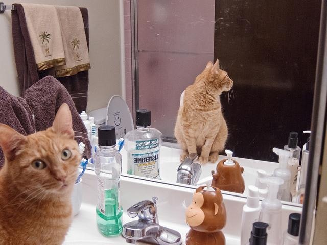
右下のように、カラーにした上で画像に重ねてみると、猫に目がいく確率が高いことがよく分かります。視点の確率が1に近いと赤、確率が0に近いと青です。
Ardizzoneの手法を実装
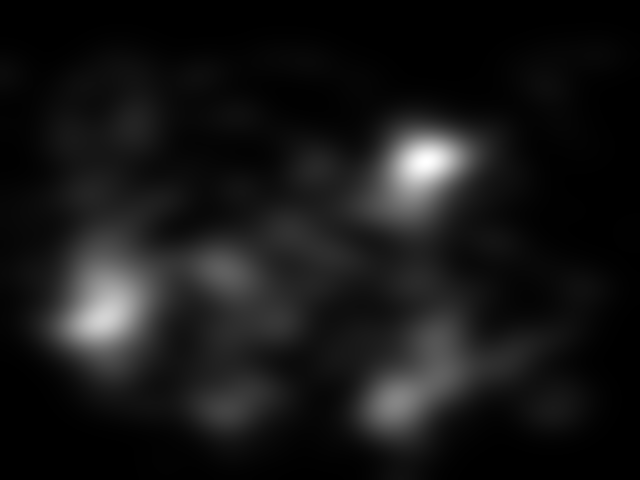
Ardizzoneの手法を実装してみます。Saliency Mapはひとまず、SALICONデータセットの学習データをそのまま使ってみることにします。こちらの猫の画像と、それに対するSaliency Mapの学習データ(正解データ)です。
どんな手法?
ある確率以上のピクセルを全て含むように切り抜こうという手法です。見られる確率が高い場所だけにしちゃおうということですね。
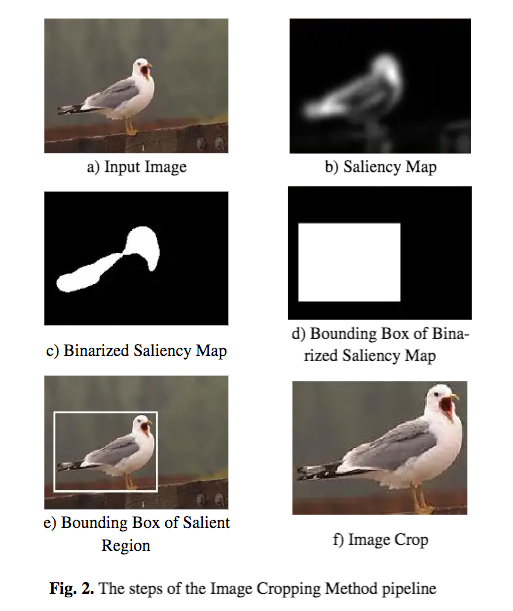
図:Ardizzoneの手法のパイプライン(論文2から引用)
この図を言葉でまとめると、以下の3ステップになります。
- Saliency Mapをある閾値で2値化する(1と0にする)
- 1の範囲を囲うバウンディングボックスを求める
- バウンディングボックスによって元の画像を切り抜く
2値化する
NumPyならば2値化は簡単です。NumPyは比較演算子(>や==)の計算もブロードキャストしてくれるため、ndarray>floatを実行すれば、各要素のTrue or Falseが手に入り2値化は完了です。
実装を見る場合はここをクリック
threshhold = 0.3 # 閾値を設定, float (0<threshhold<1)
saliencymap_path = 'COCO_train2014_000000196971.png' # Saliency Mapのパス

saliencymap = cv2.imread(saliencymap_path)[:, :, ::-1] # ndarray, (h, w, rgb), np.uint8 (0-255)
saliencymap = saliencymap[:, :, 0] # ndarray, (h, w), np.uint8 (0-255)
plt.imshow(saliencymap)
plt.show()

threshhold *= 255 # 画像から読み込んだSaliency Mapは0-255なので範囲を変換

binarized_saliencymap = saliencymap>threshhold # ndarray, (h, w), bool

plt.imshow(binarized_saliencymap)
plt.show()
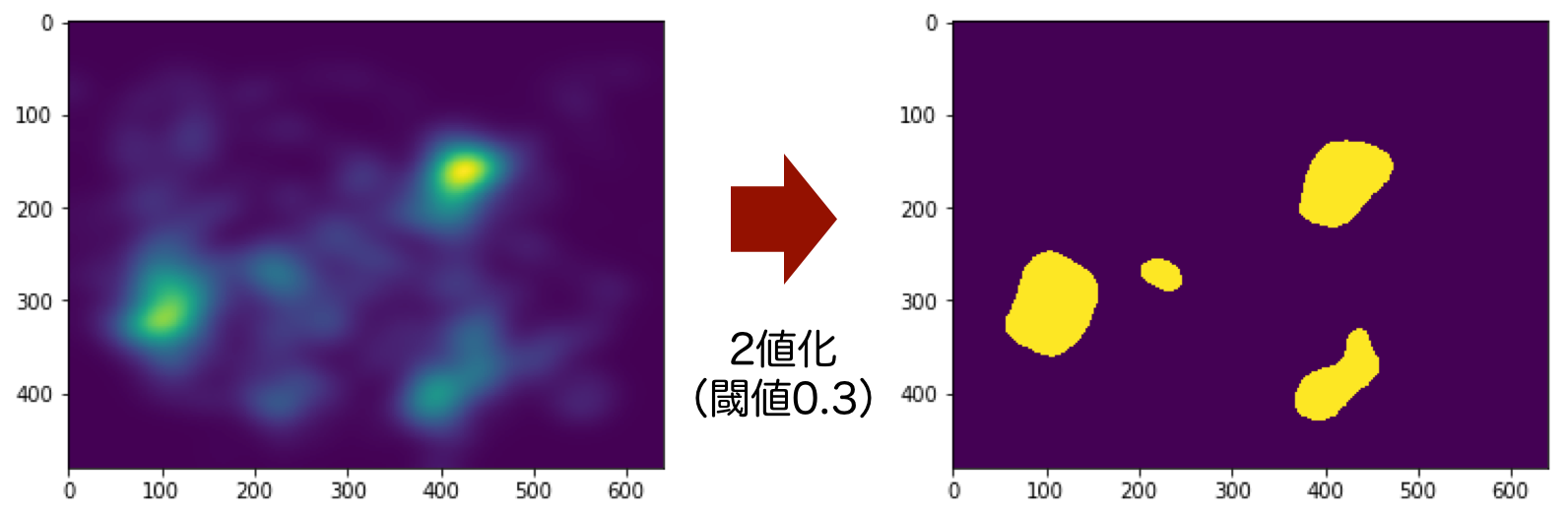
図:2値化の結果
この図のような結果になります。matplotlibのplt.imshow()のデフォルト設定で、値が大きいところが黄色、小さいところが紫で表示されています。
閾値は任意に設定できるハイパーパラメータです。今回は記事を通して0.3で統一しています。
バウンディングボックスを求める
2値化によって得た1(True)を全て含むような バウンディングボックス (ちょうど囲える矩形)を計算します。
これはOpenCVのcv2.boundingRect()に実装されていて、呼び出すだけで実現可能です。
Structural Analysis and Shape Descriptors — OpenCV 2.4.13.7 documentation
領域(輪郭)の特徴 — OpenCV-Python Tutorials 1 documentation
matplotlibにおける矩形の描画はpatches.Rectangle()を使います。
matplotlib.patches.Rectangle — Matplotlib 3.1.1 documentation
実装を見る場合はここをクリック
import matplotlib.patches as patches

# OpenCVが扱える形式に変換
binarized_saliencymap = binarized_saliencymap.astype(np.uint8) # ndarray, (h, w), np.uint8 (0 or 1)

box_x, box_y, box_width, box_height = cv2.boundingRect(binarized_saliencymap)
# box_x : int, 切り抜く左上のx座標, box_y : int, 切り抜く左上のy座標
# box_width : int, 切り抜く幅, box_height : int, 切り抜く高さ

# バウンディングボックスの描画
fig = plt.figure()
ax = plt.axes()
bounding_box = patches.Rectangle(xy=(box_x, box_y), width=box_width, height=box_height, ec='#00FF00', fill=False)
ax.imshow(binarized_saliencymap)
ax.add_patch(bounding_box)
plt.show()
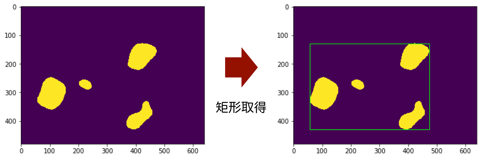
図:バウンディングボックスを取得した結果
この図のように、バウンディングボックスが取得できます。矩形の情報は左上の座標と幅・高さの値として持っています。
切り抜く
取得したバウンディングボックスに基づいて画像を切り抜きます。画像のndarrayをバウンディングボックスの値を使いスライスします。
実装を見る場合はここをクリック
image_path = 'COCO_train2014_000000196971.jpg' # 画像のパス
image = cv2.imread(image_path)[:, :, ::-1] # ndarray, (h, w, rgb), np.uint8 (0-255)

cropped_image = image[box_y:box_y+box_height, box_x:box_x+box_width] # ndarray, (h, w, rgb), np.uint8 (0-255)

# 可視化
fig = plt.figure()
ax = plt.axes()
bounding_box = patches.Rectangle(xy=(box_x, box_y), width=box_width, height=box_height, ec='#00FF00', fill=False)
ax.imshow(image)
ax.add_patch(bounding_box)
plt.show()

plt.imshow(cropped_image)
plt.show()
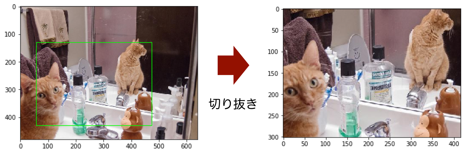
図:Ardizzoneの手法で切り抜いた結果
この図のように、視線が向きそうなところだけになった画像が得られました。
カラーにしたSaliency Mapと重ねてみる
どういう風に処理されたか分かりやすくするため、カラーにしたSaliency Mapとバウンディングボックスを画像に重ねて表示してみます。Saliency Mapをカラーにする関数と、Saliency Mapを画像に重ねる関数を実装します。
実装を見る場合はここをクリック
def color_saliencymap(saliencymap):
    """
    Saliency Mapに色をつけて可視化する。1を赤、0を青にする。

    Parameters
    ----------------
    saliencymap : ndarray, np.uint8, (h, w) or (h, w, rgb)

    Returns
    ----------------
    saliencymap_colored : ndarray, np.uint8, (h, w, rgb)
    """
    assert saliencymap.dtype==np.uint8
    assert (saliencymap.ndim == 2) or (saliencymap.ndim == 3)

    saliencymap_colored = cv2.applyColorMap(saliencymap, cv2.COLORMAP_JET)[:, :, ::-1]

    return saliencymap_colored

def overlay_saliencymap_and_image(saliencymap_color, image):
    """
    Saliency Mapと画像を重ねる。

    Parameters
    ----------------
    saliencymap_color : ndarray, (h, w, rgb), np.uint8
    image : ndarray, (h, w, rgb), np.uint8

    Returns
    ----------------
    overlaid_image : ndarray(h, w, rgb)
    """
    assert saliencymap_color.ndim==3
    assert saliencymap_color.dtype==np.uint8
    assert image.ndim==3
    assert image.dtype==np.uint8
    im_size = (image.shape[1], image.shape[0])
    saliencymap_color = cv2.resize(saliencymap_color, im_size, interpolation=cv2.INTER_CUBIC)
    overlaid_image = cv2.addWeighted(src1=image, alpha=1, src2=saliencymap_color, beta=0.7, gamma=0)
    return overlaid_image

saliencymap_colored = color_saliencymap(saliencymap) # ndarray, (h, w, rgb), np.uint8
overlaid_image = overlay_saliencymap_and_image(saliencymap_colored, image) # ndarray, (h, w, rgb), np.uint8

# 可視化
fig = plt.figure()
ax = plt.axes()
bounding_box = patches.Rectangle(xy=(box_x, box_y), width=box_width, height=box_height, ec='#00FF00', fill=False)
ax.imshow(overlaid_image)
ax.add_patch(bounding_box)
plt.show()
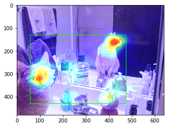
図:カラーにしたSaliency Mapとバウンディングボックスを重ねた画像
この図のように、Saliency Map上で赤くなるような視線が向く確率が高い箇所が囲えていることが分かります。
任意のアスペクト比への対応
Ardizzoneの手法では、どのようなサイズ・アスペクト比になるかはSaliency Map次第です。しかし、今はあるアスペクト比に切り抜きたいわけなので、そこを考える必要があります。
Saliency Mapの合計値が多くなるように切り抜く
これは既存の手法が見つけられなかったため、以下のアルゴリズムで切り抜く範囲を決めることにしました。
- Ardizzoneの手法で求めた範囲を全て使った上で、指定したアスペクト比になるようにある方向に範囲を伸ばす
- なお、範囲を伸ばすと画像の外に飛び出てしまう場合は、その方向は画像全体を使い、逆の方向を狭めて調整する
- 狭める範囲は、Ardizzoneの手法で求めた範囲の中で、Saliency Mapの値の合計が最大になる範囲とする
- 伸ばす範囲は、Saliency Mapの値の合計が最大になる範囲とする
ここまでで求めた範囲をできるだけ使いつつ、Saliency Mapの値の合計が最大になる範囲を探します。
クロッピングのための「SaliencyBasedImageCroppingクラス」を作り、これまでのコードを以下にまとめます。
実装を見る場合はここをクリック
import copy

import cv2
import matplotlib.pyplot as plt
import matplotlib.patches as patches
import numpy as np

class SaliencyBasedImageCropping:
    """
    Saliency Mapを利用して画像をクロッピングするためのクラス。ある閾値を超える範囲を全て使う手法[1]を利用する。

    *もしも閾値を超えるピクセルがなかった場合は、画像全体を返す。

    [1] Ardizzone, Edoardo, Alessandro Bruno, and Giuseppe Mazzola. "Saliency based image cropping." International Conference on Image Analysis and Processing. Springer, Berlin, Heidelberg, 2013.

    Parameters
    ----------------
    aspect_rate : tuple of int (x, y)
        ここでアスペクト比を指定した場合は、[1]の手法で求めた範囲をできるだけ使いつつ、Saliency Mapの値の合計が最大になる範囲を探す。
    min_size : tuple of int (w, h)
        [1]の手法で求めた範囲の各軸がこの値より小さい場合は、範囲の中心を起点に均等に範囲を広げる。

    Attributes
    ----------------
    self.aspect_rate : tuple of int (x, y)
    self.min_size : tuple of int (w, h)
    im_size : tuple of int (w, h)
    self.bounding_box_based_on_binary_saliency : list
        [1]の手法で求めた範囲
        box_x : int
        box_y : int
        box_width : int
        box_height : int
    self.bounding_box : list
        アスペクト比を調整した最終的に切り抜く範囲
        box_x : int
        box_y : int
        box_width : int
        box_height : int
    """
    def __init__(self, aspect_rate=None, min_size=(200, 200)):
        assert (aspect_rate is None)or((type(aspect_rate)==tuple)and(len(aspect_rate)==2))
        assert (type(min_size)==tuple)and(len(min_size)==2)
        self.aspect_rate = aspect_rate
        self.min_size = min_size
        self.im_size = None
        self.bounding_box_based_on_binary_saliency = None
        self.bounding_box = None

    def _compute_bounding_box_based_on_binary_saliency(self, saliencymap, threshhold):
        """
        Ardizzoneの手法[1]でSaliency Mapに基づいたクロッピング範囲を求める。

        Parameters:
        -----------------
        saliencymap : ndarray, (h, w), np.uint8
            0<=saliencymap<=255

        threshhold : float
            0<threshhold<255

        Returns:
        -----------------
        bounding_box_based_on_binary_saliency : list
            box_x : int
            box_y : int
            box_width : int
            box_height : int

        """
        assert (threshhold>0)and(threshhold<255)
        assert saliencymap.dtype==np.uint8
        assert saliencymap.ndim==2

        binarized_saliencymap = saliencymap>threshhold
        # Saliency Mapに閾値を超えるピクセルがなかったら、全てが超えた扱いにする。
        if saliencymap.sum()==0:
            saliencymap+=True
        binarized_saliencymap = (binarized_saliencymap.astype(np.uint8))*255
        # binarized_saliencymap : ndarray, (h, w), uint8, 0 or 255

        # 小さな領域はモルフォロジー処理(オープニング)によって消す
        kernel_size = round(min(self.im_size)*0.02)
        kernel = np.ones((kernel_size, kernel_size))
        binarized_saliencymap = cv2.morphologyEx(binarized_saliencymap, cv2.MORPH_OPEN, kernel)

        box_x, box_y, box_width, box_height = cv2.boundingRect(binarized_saliencymap)
        bounding_box_based_on_binary_saliency = [box_x, box_y, box_width, box_height]
        return bounding_box_based_on_binary_saliency

    def _expand_small_bounding_box_to_minimum_size(self, bounding_box):
        """
        範囲が指定したサイズより小さい場合は広げる。範囲の中心を起点に均等に範囲を広げる。画像の外に出てしまう場合はその分逆側に広げる。

        Parameters:
        -----------------
        bounding_box : list
            box_x : int
            box_y : int
            box_width : int
            box_height : int
        """
        bounding_box = copy.copy(bounding_box) # 元のリストの値を残しておきたいので深いコピー

        # axis=0 : x and witdth, axis=1 : y and hegiht
        for axis in range(2):
            if bounding_box[axis+2]<self.min_size[axis+0]:
                bounding_box[axis+0] -= np.floor((self.min_size[axis+0]-bounding_box[axis+2])/2).astype(np.int)
                bounding_box[axis+2] = self.min_size[axis+0]
                if bounding_box[axis+0]<0:
                    bounding_box[axis+0] = 0
                if (bounding_box[axis+0]+bounding_box[axis+2])>self.im_size[axis+0]:
                    bounding_box[axis+0] -= (bounding_box[axis+0]+bounding_box[axis+2]) - self.im_size[axis+0]
        return bounding_box

    def _expand_bounding_box_to_specified_aspect_ratio(self, bounding_box, saliencymap):
        """
        範囲が指定したアスペクト比になるように広げる。
        Ardizzoneの手法[1]で求めた範囲をできるだけ使いつつ、Saliency Mapの値の合計が最大になる範囲を探す。

        Parameters
        ----------------
        bounding_box : list
            box_x : int
            box_y : int
            box_width : int
            box_height : int
        saliencymap : ndarray, (h, w), np.uint8
            0<=saliencymap<=255
        """
        assert saliencymap.dtype==np.uint8
        assert saliencymap.ndim==2

        bounding_box = copy.copy(bounding_box)

        # axis=0 : x and witdth, axis=1 : y and hegiht
        if bounding_box[2]>bounding_box[3]:
            long_length_axis = 0
            short_length_axis = 1
        else:
            long_length_axis = 1
            short_length_axis = 0

        # どの方向に伸ばすか
        rate1 = self.aspect_rate[long_length_axis]/self.aspect_rate[short_length_axis]
        rate2 = bounding_box[2+long_length_axis]/bounding_box[2+short_length_axis]
        if rate1>rate2:
            moved_axis = long_length_axis
            fixed_axis = short_length_axis
        else:
            moved_axis = short_length_axis
            fixed_axis = long_length_axis

        fixed_length = bounding_box[2+fixed_axis]
        moved_length = int(round((fixed_length/self.aspect_rate[fixed_axis])*self.aspect_rate[moved_axis]))
        if moved_length > self.im_size[moved_axis]:
            # 伸ばすと画像のサイズを超えてしまう場合
            moved_axis, fixed_axis = fixed_axis, moved_axis
            fixed_length = self.im_size[fixed_axis]
            moved_length = int(round((fixed_length/self.aspect_rate[fixed_axis])*self.aspect_rate[moved_axis]))
            fixed_point = 0
            start_point = bounding_box[moved_axis]
            end_point = bounding_box[moved_axis]+bounding_box[2+moved_axis]
            if fixed_axis==0:
                saliencymap_extracted = saliencymap[start_point:end_point, :]
            elif fixed_axis==1:
                saliencymap_extracted = saliencymap[:, start_point:end_point:]
        else:
            # 伸ばして画像のサイズ内に収まる場合
            start_point = int(bounding_box[moved_axis]+bounding_box[2+moved_axis]-moved_length)
            if start_point<0:
                start_point = 0
            end_point = int(bounding_box[moved_axis]+moved_length)
            if end_point>self.im_size[moved_axis]:
                end_point = self.im_size[moved_axis]
            if fixed_axis==0:
                fixed_point = bounding_box[fixed_axis]
                saliencymap_extracted = saliencymap[start_point:end_point, fixed_point:fixed_point+fixed_length]
            elif fixed_axis==1:
                fixed_point = bounding_box[fixed_axis]
                saliencymap_extracted = saliencymap[fixed_point:fixed_point+fixed_length, start_point:end_point]
        saliencymap_summed_1d = saliencymap_extracted.sum(moved_axis)
        self.saliencymap_summed_slided = np.convolve(saliencymap_summed_1d, np.ones(moved_length), 'valid')
        moved_point = np.array(self.saliencymap_summed_slided).argmax() + start_point

        if fixed_axis==0:
            bounding_box = [fixed_point, moved_point, fixed_length, moved_length]
        elif fixed_axis==1:
            bounding_box = [moved_point, fixed_point, moved_length, fixed_length]
        return bounding_box

    def crop_center(self, image):
        """
        Saliency Mapを使わず、画像の中心を指定したアスペクト比でクロッピングする。

        Parameters:
        -----------------
        image : ndarray, (h, w, rgb), uint8

        Returns:
        -----------------
        cropped_image : ndarray, (h, w, rgb), uint8
        """
        assert image.dtype==np.uint8
        assert image.ndim==3

        im_size = (image.shape[1], image.shape[0]) # tuple of int, (width, height)
        center = (int(round(im_size[0]/2)), int(round(im_size[1]/2))) # tuple of int, (x, y)

        if im_size[0]>im_size[1]:
            box_y = 0
            box_height = im_size[1]
            box_width = int(round((im_size[1]/self.aspect_rate[1])*self.aspect_rate[0]))
            if box_width>im_size[0]:
                box_x = 0
                box_width = im_size[0]
                box_height = int(round((im_size[0]/self.aspect_rate[0])*self.aspect_rate[1]))
                box_y = int(round(center[1]-(box_height/2)))
            else:
                box_x = int(round(center[0]-(box_width/2)))

        else:
            box_x = 0
            box_width = im_size[0]
            box_height = int(round((im_size[0]/self.aspect_rate[0])*self.aspect_rate[1]))
            if box_height>im_size[1]:
                box_y = 0
                box_height = im_size[1]
                box_width = int(round((im_size[1]/self.aspect_rate[1])*self.aspect_rate[0]))
                box_y = int(round(center[0]-(box_width/2)))
            else:
                box_y = int(round(center[1]-(box_height/2)))

        cropped_image = image[box_y:box_y+box_height, box_x:box_x+box_width]
        return cropped_image

    def crop(self, image, saliencymap, threshhold=0.3):
        """
        Saliency Mapを用いてクロッピングする。

        Parameters:
        -----------------
        image : ndarray, (h, w, rgb), np.uint8
        saliencymap : ndarray, (h, w), np.uint8
            Saliency map's ndarray need not be the same size as image's ndarray. Saliency map is resized within this method.
        threshhold : float
            0 < threshhold <1

        Returns:
        -----------------
        cropped_image : ndarray, (h, w, rgb), uint8
        """
        assert (threshhold>0)and(threshhold<1)
        assert image.dtype==np.uint8
        assert image.ndim==3
        assert saliencymap.dtype==np.uint8
        assert saliencymap.ndim==2

        threshhold = threshhold*255 # scale to 0 - 255
        self.im_size = (image.shape[1], image.shape[0]) # (width, height)
        saliencymap = cv2.resize(saliencymap, self.im_size, interpolation=cv2.INTER_CUBIC)

        # compute bounding box based on saliency map
        bounding_box_based_on_binary_saliency = self._compute_bounding_box_based_on_binary_saliency(saliencymap, threshhold)
        bounding_box = self._expand_small_bounding_box_to_minimum_size(bounding_box_based_on_binary_saliency)
        if self.aspect_rate is not None:
            bounding_box = self._expand_bounding_box_to_specified_aspect_ratio(bounding_box, saliencymap)

        box_y = bounding_box[1]
        box_x = bounding_box[0]
        box_height = bounding_box[3]
        box_width = bounding_box[2]

        cropped_image = image[box_y:box_y+box_height, box_x:box_x+box_width]

        self.bounding_box_based_on_binary_saliency = bounding_box_based_on_binary_saliency
        self.bounding_box  = bounding_box

        return cropped_image

# -------------------
# SETTING
threshhold = 0.3 # 閾値を設定, float (0<threshhold<1)
saliencymap_path = 'COCO_train2014_000000196971.png' # Saliency Mapのパス
image_path = 'COCO_train2014_000000196971.jpg' # 画像のパス
# -------------------

saliencymap = cv2.imread(saliencymap_path)[:, :, ::-1] # ndarray, (h, w, rgb), np.uint8 (0-255)
saliencymap = saliencymap[:, :, 0] # ndarray, (h, w), np.uint8 (0-255)
image = cv2.imread(image_path)[:, :, ::-1] # ndarray, (h, w, rgb), np.uint8 (0-255)

# Saliency Mapを用いてクロップした画像の可視化
cropper = SaliencyBasedImageCropping(aspect_rate=(1, 3))
cropped_image = cropper.crop(image, saliencymap, threshhold=0.3)
plt.imshow(cropped_image)
plt.show()

# Saliency Mapとバウンディングボックスの可視化
# 指定したアスペクト比に合わせたものが赤、合わせる前が緑
saliencymap_colored = color_saliencymap(saliencymap) # ndarray, (h, w, rgb), np.uint8
overlaid_image = overlay_saliencymap_and_image(saliencymap_colored, image) # ndarray, (h, w, rgb), np.uint8
box_x, box_y, box_width, box_height = cropper.bounding_box
box_x_0, box_y_0, box_width_0, box_height_0 = cropper.bounding_box_based_on_binary_saliency
fig = plt.figure()
ax = plt.axes()
bounding_box = patches.Rectangle(xy=(box_x, box_y), width=box_width, height=box_height, ec='#FF0000', fill=False)
bounding_box_based_on_binary_saliency = patches.Rectangle(xy=(box_x_0, box_y_0), width=box_width_0, height=box_height_0, ec='#00FF00', fill=False)
ax.imshow(overlaid_image)
ax.add_patch(bounding_box)
ax.add_patch(bounding_box_based_on_binary_saliency)
plt.show()

# 比較として中心をクロップした画像の可視化
center_cropped_image = cropper.crop_center(image)
plt.imshow(center_cropped_image)
plt.show()
Saliency Mapが最大値になる範囲を見つける上では、np.convolve()を利用しています。
numpy.convolve — NumPy v1.17 Manual
これは1次元の畳み込みを行う関数です。合計したい長さの全て1の配列と畳み込むことで、以下のように一定の範囲ごとの合計を計算できます。
array_1d = np.array([1, 2, 3, 4])
print(np.convolve(array_1d, np.ones(2), 'valid')) # [3. 5. 7.]
単純なPython上のfor文を使うと速度が低下するため、極力NumPyの関数を組み合わせていきます。
その他、2値化の処理において、非常に小さい領域をモルフォロジー変換によって消す実装を加えています。特にこの後深層学習によってSaliency Mapを求めた時に、そういった領域が発生しやすいためこの実装を加えています。
モルフォロジー変換 — OpenCV-Python Tutorials 1 documentation
結果を見る
アスペクト比を調整する前を緑のバウンディングボックス、調整した後を赤のバウンディングボックスで示します。
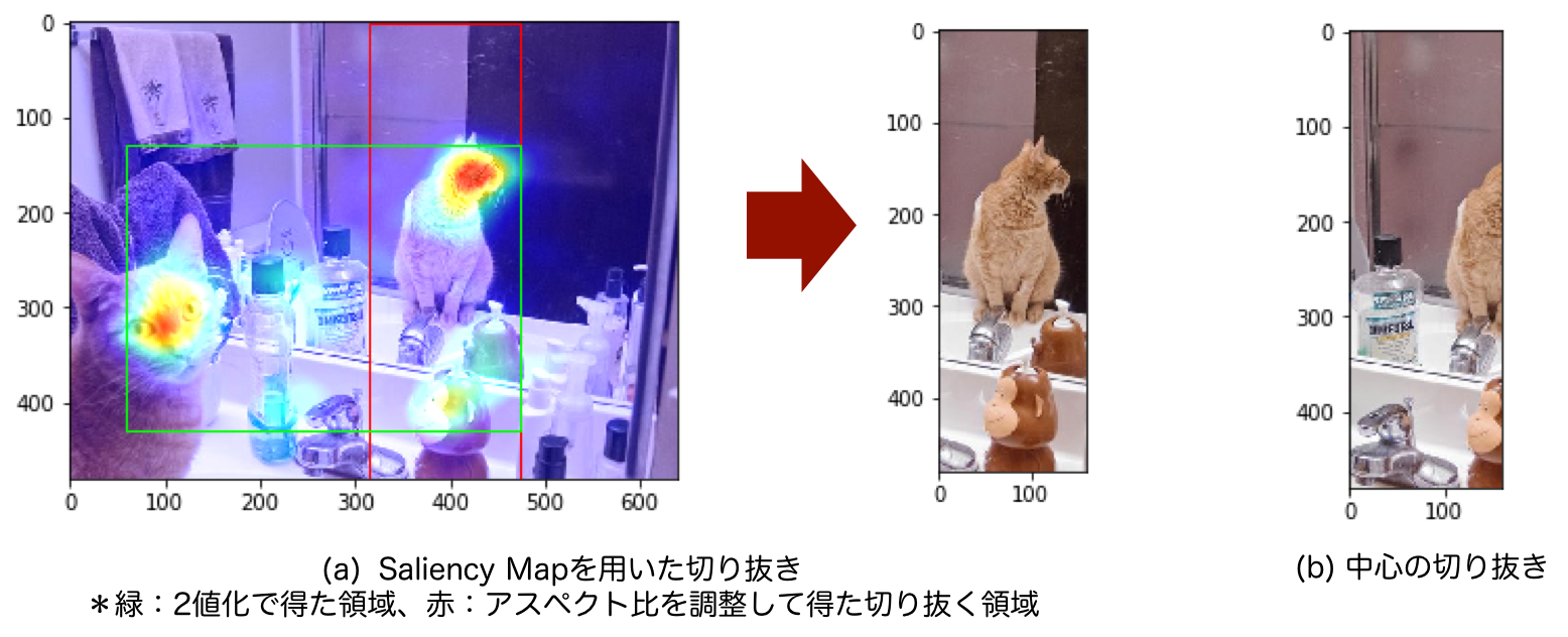
図:Saliency Mapを用いて1:3のアスペクト比で切り抜いた結果
この図(a)のように、縦長の範囲の中に猫とハンドソープ?を入れて切り抜くことに成功しました。最初に実装した中心を切り抜いただけの図(b)と比べても、人間が見たいところが良い感じに入れられています。
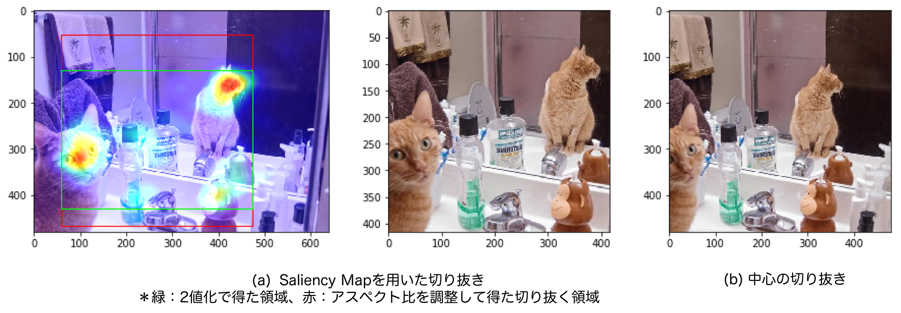
図:Saliency Mapを用いて1:1のアスペクト比で切り抜いた結果
正方形(1:1)の場合はこのようになります。中心を切り抜いた場合(図(b))もしっかりと猫が入っていますが、Saliency Mapを使った場合(図(a))の方が狭い範囲を切り抜いているので、同じ大きさで表示した場合、猫が大きくなっています。ある物体が写っているかだけでなく、十分な大きさで写っているかもクロッピングにおいては重要になります。
Saliency Mapを深層学習を用いて推定するモデル(SalGAN)をPyTorchで実装
ここまでだけでは自分で用意した画像をクロッピングすることはできません。SALICONデータセットの画像ではなく、自分で撮影したクリスマスツリーの画像を良い感じに切り抜きたいので、深層学習を使ってSaliency Mapを推定モデルを作っていきます。
Saliency Mapタスクのベンチマークサイト「MIT Saliency Benchmark」4を見るといろいろな手法が並んでいますが、今回はその中でもSalGAN5を実装してみることにします。スコアはあまり高くないようですが、仕組みがシンプルに見えたのでこれを選びました。
著者実装6も公開されていましたが、フレームワークがLasagne(Theano)であまり馴染みがないので、参考にしつつPyTorchで書いていきます。
SalGANはどんなもの?
「SalGAN: Visual Saliency Prediction with Generative Adversarial Networks」は2017年に発表された論文です。名前の通り、GAN(Generative Adversarial Networks) を使ってSaliency Mapを推定しようという手法です。
GANについての説明は既に分かりやすい記事がたくさんあるため省略します。例えば 今さら聞けないGAN(1) 基本構造の理解 - Qiita がおすすめです。実装や説明が充実している代表的なGANの手法が分かれば、それとの違いを考えることで実装できます。
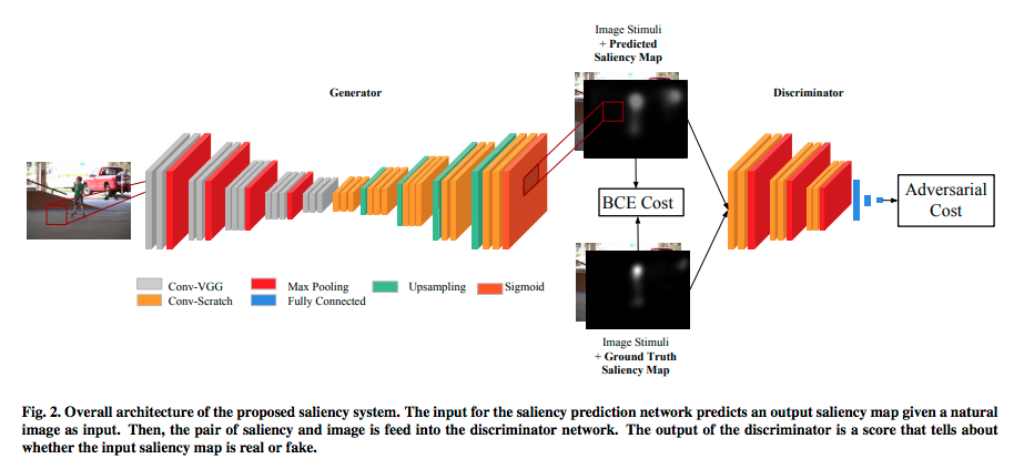
図:SalGANの全体構造(論文5から引用)
Saliency Mapは各ピクセルに対して視点がある確率(0から1)なので、ピクセルごとの2値分類問題と言えます。1クラスのセグメンテーションに近いです。画像を入力して画像(Saliency Map)を出力したいため、この図にあるようにCNNを使った Encoder-Decoderモデル になります。GANを使った画像対画像というとPix2Pix7が有名ですが、そちらのようなU-Net構造にはなっていません。
Encoder-Decoderモデルでは出力したSaliency Mapと、正解データの Binary Cross Entropy を小さくするように学習することもできます。しかし、このSalGANはそれに加えて、Saliency Mapを正解データなのか、推定したものなのか分類するネットワーク(Discriminator)を加えることで、より精度を上げようとしています。
Encoder-Decoder部分(Generator)の損失関数は次のようになります。通常のAdversarial Lossの他に、推定したSaliency Mapと正解データのBinary Cross Entropyの項が加わります。割合をハイパーパラメータ$\alpha$で調整します。
$$
\mathcal{L}_{BCE} = -\frac{1}{N}\sum_{j=1}^{N}(S_{j}\log{(\hat{S}_{j})}+(1-S_{j})\log{(1-\hat{S}_{j})}).
$$
$$
\mathcal{L} = \alpha\cdot\mathcal{L}_{BCE} + L(D(I, \hat{S}), 1).
$$
Discriminatorの損失関数は次のようになります。一般的な形です。
$$
\mathcal{L}_{\mathcal{D}} = L(D(I, S), 1)+L(D(I, \hat{S}),0).
$$
もう少し読み解く
論文を引用しつつ、実装に必要な情報を読み解いていきます。全体構造を見てなんとなく分かったけど、もう少し知っておきたい情報が書いてある箇所を探します。
The encoder part of the network is identical in architecture to VGG-16 (Simonyan and Zisserman, 2015), omitting the final pooling and fully connected layers. The network is initialized with the weights of a VGG-16 model trained on the ImageNet data set for object classification (Deng et al., 2009). Only the last two groups of convolutional layers in VGG-16 are modified during the training for saliency prediction, while the earlier layers remain fixed from the original VGG-16 model.
- GeneratorのEncoder部分のCNNはVGG16を使う
- 最後のプーリング層と全結合層は除く
- ImageNetで学習した重みを初期値とする
- 後ろの2グループの畳み込み層だけ学習する
- 前の3グループの畳み込み層の重みはImageNetで学習した重みのまま固定する
The decoder architecture is structured in the same way as the encoder, but with the ordering of layers reversed, and with pooling layers being replaced by upsampling layers. Again, ReLU non-linearities are used in all convolution layers, and a final 1 × 1 convolution layer with sigmoid non-linearity is added to
produce the saliency map. The weights for the decoder are randomly initialized. The final output of the network is a saliency map in the same size to input image.
- DecoderはEncoderと同じだが、プーリング層の代わりにアップサンプリング層を入れる
- 最後の層は1x1の畳み込みの後にシグモイド関数とする
- 重みはランダムに初期化する
- 出力は入力と同じサイズになる
The input to the discriminator network is an RGBS image of size 256×192×4 containing both the source
image channels and (predicted or ground truth) saliency.
- DiscriminatorへはSaliency Mapだけでなく元の画像も結合して4チャンネルで入力する
- そもそも画像は256×192で入力する
We train the networks on the 15,000 images from the SALICON training set using a batch size of 32.
- SALICONデータセットの15000枚の画像を使う
- バッチサイズは32とする
なお、今回は論文の再現実験を行いたいわけではないので、実装にあたり細部にはこだわっていません。例えば論文内のReLUの代わりに、一般的に使うと効果的だとされるLeakyReLUを採用するなどしています。
コードを書く
コードを書いていきます。基本はCNNによるEncoder-DecoderモデルのGANなので、既存の似た手法の実装を参考にしていきます。例えばeriklindernorenさんのGitHubはPyTorchで各種GANが実装されたものが公開されています。DCGANの実装8など良さそうです。
GeneratorとDiscriminatorのクラスを作る
GeneratorではImageNetで学習済みのVGG16を使いますが、これはtorchvision[^9]に用意されています。SalGANでは前側は重みを固定、後ろは学習ということなので、torchvision.models.vgg16(pretrained=True).features[:17]のように層を分けて記述します。何番目が何の層なのかはprint(torchvision.models.vgg16(pretrained=True).features)で確認できます。
torchvision.models — PyTorch master documentation
実装を見る場合はここをクリック
from torch import nn
import torchvision

class Generator(nn.Module):
    def __init__(self, pretrained=True):
        super().__init__()
        self.encoder_first = torchvision.models.vgg16(pretrained=True).features[:17] # 重み固定して使う部分
        self.encoder_last = torchvision.models.vgg16(pretrained=True).features[17:-1] # 学習する部分
        self.decoder = nn.Sequential(
                    nn.Conv2d(512, 512, 3, padding=1),
                    nn.LeakyReLU(),
                    nn.Conv2d(512, 512, 3, padding=1),
                    nn.LeakyReLU(),
                    nn.Conv2d(512, 512, 3, padding=1),
                    nn.LeakyReLU(),
                    nn.Upsample(scale_factor=2),
                    nn.Conv2d(512, 512, 3, padding=1),
                    nn.LeakyReLU(),
                    nn.Conv2d(512, 512, 3, padding=1),
                    nn.LeakyReLU(),
                    nn.Conv2d(512, 512, 3, padding=1),
                    nn.LeakyReLU(),
                    nn.Upsample(scale_factor=2),
                    nn.Conv2d(512, 256, 3, padding=1),
                    nn.LeakyReLU(),
                    nn.Conv2d(256, 256, 3, padding=1),
                    nn.LeakyReLU(),
                    nn.Conv2d(256, 256, 3, padding=1),
                    nn.LeakyReLU(),
                    nn.Upsample(scale_factor=2),
                    nn.Conv2d(256, 128, 3, padding=1),
                    nn.LeakyReLU(),
                    nn.Conv2d(128, 128, 3, padding=1),
                    nn.LeakyReLU(),
                    nn.Upsample(scale_factor=2),
                    nn.Conv2d(128, 64, 3, padding=1),
                    nn.LeakyReLU(),
                    nn.Conv2d(64, 64, 3, padding=1),
                    nn.LeakyReLU(),
                    nn.Conv2d(64, 1, 1, padding=0),
                    nn.Sigmoid())

    def forward(self, x):
        x = self.encoder_first(x)
        x = self.encoder_last(x)
        x = self.decoder(x)
        return x

class Discriminator(nn.Module):
    def __init__(self):
        super().__init__()
        self.main = nn.Sequential(
                    nn.Conv2d(4, 3, 1, padding=1),
                    nn.LeakyReLU(inplace=True),
                    nn.Conv2d(3, 32, 3, padding=1),
                    nn.LeakyReLU(inplace=True),
                    nn.MaxPool2d(2, stride=2),
                    nn.Conv2d(32, 64, 3, padding=1),
                    nn.LeakyReLU(inplace=True),
                    nn.Conv2d(64, 64, 3, padding=1),
                    nn.LeakyReLU(inplace=True),
                    nn.MaxPool2d(2, stride=2),
                    nn.Conv2d(64, 64, 3, padding=1),
                    nn.LeakyReLU(inplace=True),
                    nn.Conv2d(64, 64, 3, padding=1),
                    nn.LeakyReLU(inplace=True),
                    nn.MaxPool2d(2, stride=2))
        self.classifier = nn.Sequential(
                    nn.Linear(64*32*24, 100, bias=True),
                    nn.Tanh(),
                    nn.Linear(100, 2, bias=True),
                    nn.Tanh(),
                    nn.Linear(2, 1, bias=True),
                    nn.Sigmoid())

    def forward(self, x):
        x = self.main(x)
        x = x.view(x.shape[0], -1)
        x = self.classifier(x)
        return x
データセットクラスを作る
SALICONデータセットを読み込むためのデータセットクラスが必要です。用意したデータセットとタスクに合わせて記述するのがやや面倒な箇所です。どう書くんだっけとなった時はPyTorchのチュートリアルが参考になります。
Writing Custom Datasets, DataLoaders and Transforms — PyTorch Tutorials 1.3.1 documentation
ここにtorchvision.transformsを使った前処理も記述します。今回は192×256へのリサイズと、Normalizeだけ行います。
torchvision.transforms — PyTorch master documentation
なお、SALICONデータセットはLSUN’17 Saliency Prediction Challenge | SALICONからダウンロード可能です。
実装を見る場合はここをクリック
import os

import torch.utils.data as data
import torchvision.transforms as transforms

class SALICONDataset(data.Dataset):
    def __init__(self, root_dataset_dir, val_mode = False):
        """
        SALICONデータセットを読み込むためのDatasetクラス

        Parameters:
        -----------------
        root_dataset_dir : str
            SALICONデータセットの上のディレクトリのパス
        val_mode : bool (default: False)
            FalseならばTrainデータを、TrueならばValidationデータを読み込む
        """
        self.root_dataset_dir = root_dataset_dir
        self.imgsets_dir = os.path.join(self.root_dataset_dir, 'SALICON/image_sets')
        self.img_dir = os.path.join(self.root_dataset_dir, 'SALICON/imgs')
        self.distribution_target_dir = os.path.join(self.root_dataset_dir, 'SALICON/algmaps')
        self.img_tail = '.jpg'
        self.distribution_target_tail = '.png'
        self.transform = transforms.Compose([transforms.Resize((192, 256)), transforms.ToTensor(), transforms.Normalize([0.5], [0.5])])
        self.distribution_transform = transforms.Compose([transforms.Resize((192, 256)), transforms.ToTensor()])

        if val_mode:
            train_or_val = "val"
        else:
            train_or_val = "train"
        imgsets_file = os.path.join(self.imgsets_dir, '{}.txt'.format(train_or_val))
        files = []
        for data_id in open(imgsets_file).readlines():
            data_id = data_id.strip()
            img_file = os.path.join(self.img_dir, '{0}{1}'.format(data_id, self.img_tail))
            distribution_target_file = os.path.join(self.distribution_target_dir, '{0}{1}'.format(data_id, self.distribution_target_tail))
            files.append({
                'img': img_file,
                'distribution_target': distribution_target_file,
                'data_id': data_id
            })
        self.files = files

    def __len__(self):
        return len(self.files)

    def __getitem__(self, index):
        """
        Returns
        -----------
        data : list
            [img, distribution_target, data_id]
        """
        data_file = self.files[index]
        data = []

        img_file = data_file['img']
        img = Image.open(img_file)
        data.append(img)

        distribution_target_file = data_file['distribution_target']
        distribution_target = Image.open(distribution_target_file)
        data.append(distribution_target)

        # transform
        data[0] = self.transform(data[0])
        data[1] = self.distribution_transform(data[1])

        data.append(data_file['data_id'])
        return data
学習する
残りの学習のためのコードを書きます。損失関数の計算と、GeneratorとDiscriminatorの学習方法をどうするかがポイントです。
論文と同じ120エポックの学習にGPUを使用して数時間程度です。
実装を見る場合はここをクリック
from datetime import datetime

import torch
from torch.autograd import Variable

# -----------------
# SETTING
root_dataset_dir = "" # SALICONデータセットの上のディレクトリのパス
alpha = 0.005 # Generatorの損失関数のハイパーパラメータ。論文の推奨値は0.005
epochs = 120
batch_size = 32 # 論文では32
# -----------------

# 開始時間をファイル名に利用
start_time_stamp = '{0:%Y%m%d-%H%M%S}'.format(datetime.now())

save_dir = "./log/"
if not os.path.exists(save_dir):
    os.makedirs(save_dir)

DEVICE = torch.device("cuda:0" if torch.cuda.is_available() else "cpu")

# データローダーの読み込み
train_dataset = SALICONDataset(
                    root_dataset_dir,
                )
train_loader = torch.utils.data.DataLoader(train_dataset, batch_size = batch_size, shuffle=True, num_workers = 4, pin_memory=True, sampler=None)
val_dataset = SALICONDataset(
                    root_dataset_dir,
                    val_mode=True
                )
val_loader = torch.utils.data.DataLoader(val_dataset, batch_size = 1, shuffle=False, num_workers = 4, pin_memory=True, sampler=None)

# モデルと損失関数の読み込み
loss_func = torch.nn.BCELoss().to(DEVICE)
generator = Generator().to(DEVICE)
discriminator = Discriminator().to(DEVICE)

# 最適化手法の定義(論文中の設定を使用)
optimizer_G = torch.optim.Adagrad([
                {'params': generator.encoder_last.parameters()},
                {'params': generator.decoder.parameters()}
            ], lr=0.0001, weight_decay=3*0.0001)
optimizer_D = torch.optim.Adagrad(discriminator.parameters(), lr=0.0001, weight_decay=3*0.0001)

# 学習
for epoch in range(epochs):
    n_updates = 0 # イテレーションのカウント
    n_discriminator_updates = 0
    n_generator_updates = 0
    d_loss_sum = 0
    g_loss_sum = 0

    for i, data in enumerate(train_loader):
        imgs = data[0] # ([batch_size, rgb, h, w])
        salmaps = data[1] # ([batch_size, 1, h, w])

        # Discriminator用のラベルを作成
        valid = Variable(torch.FloatTensor(imgs.shape[0], 1).fill_(1.0), requires_grad=False).to(DEVICE)
        fake = Variable(torch.FloatTensor(imgs.shape[0], 1).fill_(0.0), requires_grad=False).to(DEVICE)

        imgs = Variable(imgs).to(DEVICE)
        real_salmaps = Variable(salmaps).to(DEVICE)

        # イテレーションごとにGeneratorとDiscriminatorを交互に学習
        if n_updates % 2 == 0:
            # -----------------
            #  Train Generator
            # -----------------

            optimizer_G.zero_grad()
            gen_salmaps = generator(imgs)

            # Discriminatorへの入力用に元の画像と生成したSaliency Mapを結合して4チャンネルの配列を作る
            fake_d_input = torch.cat((imgs, gen_salmaps.detach()), 1) # ([batch_size, rgbs, h, w])

            # Generatorの損失関数を計算
            g_loss1 = loss_func(gen_salmaps, real_salmaps)
            g_loss2 = loss_func(discriminator(fake_d_input), valid)
            g_loss = alpha*g_loss1 + g_loss2

            g_loss.backward()
            optimizer_G.step()

            g_loss_sum += g_loss.item()
            n_generator_updates += 1

        else:
            # ---------------------
            #  Train Discriminator
            # ---------------------

            optimizer_D.zero_grad()

            # Discriminatorへの入力用に元の画像と正解データのSaliency Mapを結合して4チャンネルの配列を作る
            real_d_input = torch.cat((imgs, real_salmaps), 1) # ([batch_size, rgbs, h, w])

            # Discriminatorの損失関数を計算
            real_loss = loss_func(discriminator(real_d_input), valid)
            fake_loss = loss_func(discriminator(fake_d_input), fake)
            d_loss = (real_loss + fake_loss) / 2

            d_loss.backward()
            optimizer_D.step()

            d_loss_sum += d_loss.item()
            n_discriminator_updates += 1

        n_updates += 1
        if n_updates%10==0:
            if n_discriminator_updates>0:
                print(
                    "[%d/%d (%d/%d)] [loss D: %f, G: %f]"
                    % (epoch, epochs-1, i, len(train_loader), d_loss_sum/n_discriminator_updates , g_loss_sum/n_generator_updates)
                )
            else:
                print(
                    "[%d/%d (%d/%d)] [loss G: %f]"
                    % (epoch, epochs-1, i, len(train_loader), g_loss_sum/n_generator_updates)
                )

    # 重みの保存
    # 5エポックごとと、最後のエポックを保存する
    if ((epoch+1)%5==0)or(epoch==epochs-1):
        generator_save_path = '{}.pkl'.format(os.path.join(save_dir, "{}_generator_epoch{}".format(start_time_stamp, epoch)))
        discriminator_save_path = '{}.pkl'.format(os.path.join(save_dir, "{}_discriminator_epoch{}".format(start_time_stamp, epoch)))
        torch.save(generator.state_dict(), generator_save_path)
        torch.save(discriminator.state_dict(), discriminator_save_path)

    # エポックごとにValidationデータの一部を可視化
    with torch.no_grad():
        print("validation")
        for i, data in enumerate(val_loader):
            image = Variable(data[0]).to(DEVICE)
            gen_salmap = generator(imgs)
            gen_salmap_np = np.array(gen_salmaps.data.cpu())[0, 0]

            plt.imshow(np.array(image[0].cpu()).transpose(1, 2, 0))
            plt.show()
            plt.imshow(gen_salmap_np)
            plt.show()
            if i==1:
                break
Saliency Mapを推定する
学習したSalGANに画像を入力し、Saliency Mapを推定してみます。学習に使っていない画像でどう推定されるかを見ます。
実装を見る場合はここをクリック
generator_path = "" # 学習して得たGeneratorの重みファイル(pkl)のパス
image_path = "COCO_train2014_000000196971.jpg" # 入力したい画像のパス

generator = Generator().to(DEVICE)
generator.load_state_dict(torch.load(generator_path))

image_pil = Image.open(image_path) # transformに対してはPIL形式の画像の入力を想定している
image = np.array(image_pil)
plt.imshow(image)
plt.show()

transform = transforms.Compose([transforms.Resize((192, 256)), transforms.ToTensor(), transforms.Normalize([0.5], [0.5])])
image_torch = transform(image_pil)
image_torch = image_torch.unsqueeze(0).to(DEVICE) # (1, rgb, h, w)
with torch.no_grad():
    pred_saliencymap = generator(img_torch)
    pred_saliencymap = np.array(pred_saliencymap.cpu())[0, 0]
pred_saliencymap = pred_saliencymap/pred_saliencymap.sum() # 和が1になるようにスケーリング
pred_saliencymap = ((pred/pred.max())*255).astype(np.uint8) # 画像として扱えるようにnp.uint8に変換
plt.imshow(pred_saliencymap)
plt.show()
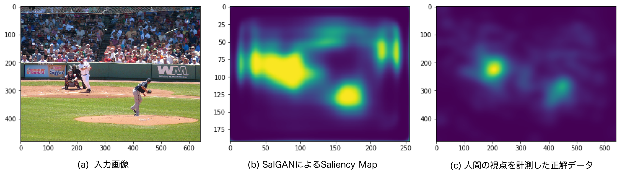
図:SalGANで推定したSaliency Mapの例
この図(b)のSaliency Mapが推定できました。正解データ(図(c))と比べると大味な印象はありますが、ピッチャーとバッター周辺の納得できる箇所の確率が高く推定できています。
しっかりと学習させる場合、論文内で行われているようにSaliency Mapのための様々な指標で検証する必要があります。今は検証していないため、論文で紹介されているSalGANと比べどの程度の結果が得られているかは不明です。今回はクロッピングすることがメインなため、定性的にそれっぽいものができたということで先に進みたいと思います。
推定したSaliency Mapで画像を切り抜く
これで作りたかったものができました。SalGANで推定したSaliency Mapをクロッピングのクラスと組み合わせることで、画像を良い感じに切り抜きます。
実装を見る場合はここをクリック
# -------------------
# SETTING
threshhold = 0.3 # 閾値を設定, float (0<threshhold<1)
generator_path = "" # 学習して得たGeneratorの重みファイル(pkl)のパス
image_path = "COCO_train2014_000000196971.jpg" # 切り抜きたい画像のパス
# -------------------

generator = Generator().to(DEVICE)
generator.load_state_dict(torch.load(generator_path))

image_pil = Image.open(image_path) # transformに対してはPIL形式の画像の入力を想定している
image = np.array(image_pil)
plt.imshow(image)
plt.show()

transform = transforms.Compose([transforms.Resize((192, 256)), transforms.ToTensor(), transforms.Normalize([0.5], [0.5])])
image_torch = transform(image_pil)
image_torch = image_torch.unsqueeze(0).to(DEVICE) # (1, rgb, h, w)
with torch.no_grad():
    pred_saliencymap = generator(image_torch)
    pred_saliencymap = np.array(pred_saliencymap.cpu())[0, 0]
pred_saliencymap = pred_saliencymap/pred_saliencymap.sum() # 和が1になるようにスケーリング
pred_saliencymap = ((pred_saliencymap/pred_saliencymap.max())*255).astype(np.uint8) # 画像として扱えるようにnp.uint8に変換
plt.imshow(pred_saliencymap)
plt.show()

# Saliency Mapを用いてクロップした画像の可視化
cropper = SaliencyBasedImageCropping(aspect_rate=(1, 3))
cropped_image = cropper.crop(image, pred_saliencymap, threshhold=0.3)
plt.imshow(cropped_image)
plt.show()

# Saliency Mapとバウンディングボックスの可視化
# 指定したアスペクト比に合わせたものが赤、合わせる前が緑
saliencymap_colored = color_saliencymap(pred_saliencymap) # ndarray, (h, w, rgb), np.uint8
overlaid_image = overlay_saliencymap_and_image(saliencymap_colored, image) # ndarray, (h, w, rgb), np.uint8
box_x, box_y, box_width, box_height = cropper.bounding_box
box_x_0, box_y_0, box_width_0, box_height_0 = cropper.bounding_box_based_on_binary_saliency
fig = plt.figure()
ax = plt.axes()
bounding_box = patches.Rectangle(xy=(box_x, box_y), width=box_width, height=box_height, ec='#FF0000', fill=False)
bounding_box_based_on_binary_saliency = patches.Rectangle(xy=(box_x_0, box_y_0), width=box_width_0, height=box_height_0, ec='#00FF00', fill=False)
ax.imshow(overlaid_image)
ax.add_patch(bounding_box)
ax.add_patch(bounding_box_based_on_binary_saliency)
plt.show()

# 比較として中心をクロップした画像の可視化
center_cropped_image = cropper.crop_center(image)
plt.imshow(center_cropped_image)
plt.show()
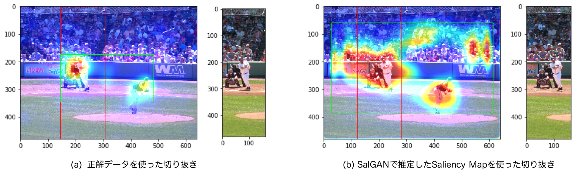
図:正解データを使った場合とSalGANを使った場合の切り抜きの比較(野球の画像)
図(a)の正解データを使った場合と、図(b)のSalGANを使った場合で、どちらもバッター部分を切り抜くというほぼ同じ結果が得られました。バッターとピッチャーどちらにより視線が向くか?ということを十分に学習できているというわけでもなさそうですが、同じように切り抜けたのは嬉しいですね。
この手の話は、うまくいった結果だけ載せているcherry pickingなのでは?という疑問がつきまといます。この成果を定量的に測るのであれば、SALICONデータセットに対してこの2種類の重なり具合を見ることができるかと思います。物体検出タスクにおけるIoUのような計算です。しかし、今はあくまで作ってみたよという話なので割愛します。
記事の前半で登場した猫の画像、可愛いから使っていましたが実はTrainデータなため、検証には不適切です。でも一応見ておきましょう。
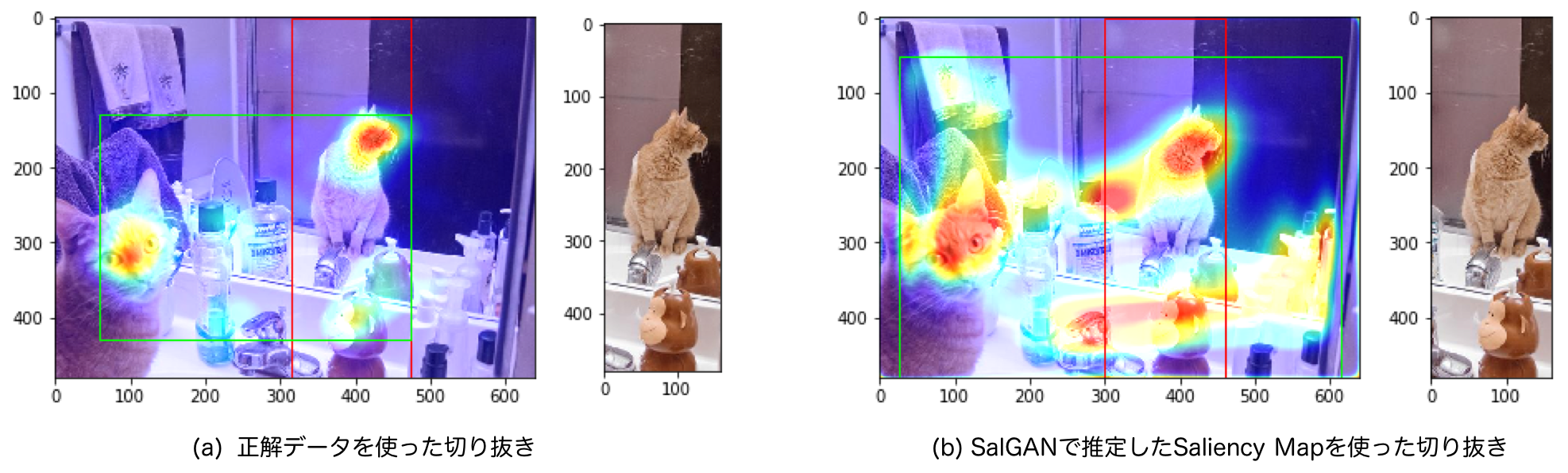
図:正解データを使った場合とSalGANを使った場合の切り抜きの比較(猫の画像)
こちらもほぼ同じような結果が得られました。良かったです。
クリスマスツリーを切り抜く
ついに最初のクリスマスツリーの画像に戻ります。データセットにない、自分で撮った写真で、自分が納得な切り抜きができれば目的達成です。
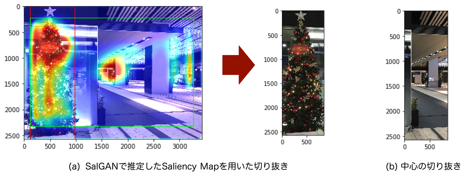
図:SalGANを使った場合と単純に中心とした場合の切り抜きの比較(クリスマスツリーの画像)
完璧な結果が得られました。クリスマスツリーの写った図(a)は、写っていない図(b)よりも良い感じですね。AI?の力で人がやる場合に近いことを自動で行える仕組みが完成しました。これで何も写ってない所が切り取られてがっかりすることが減ったり、人力で画像を切り抜き続ける仕事が減ったりするかもしれません。
まとめ
Saliency Mapを使ったクロッピング2と、Saliency Mapを推定するSalGAN5の2本の論文の実装+アルファというような内容でした。
公開されている情報だけでこんなものも作れるわけです。深層学習や機械学習でチュートリアル的なものを動かして止まっていた人も、ちょっと挑戦してこんな風に何か作ってみてもらいたいなと思います!
-
画像を最適かつ自動的にトリミングするニューラルネットワークのご紹介 https://blog.twitter.com/ja_jp/topics/product/2018/0125ML-CR.html ↩
-
E. Ardizzone, A. Bruno, G. Mazzola, Saliency Based Image Cropping, ICIAP, 2013 https://www.academia.edu/35825403/Saliency_based_image_cropping ↩ ↩2 ↩3
-
SALICON http://salicon.net/ ↩
-
MIT Saliency Benchmark http://saliency.mit.edu/results_mit300.html ↩
-
Pan, Junting, et al. "Salgan: Visual saliency prediction with generative adversarial networks." arXiv preprint arXiv:1701.01081 (2017). https://arxiv.org/abs/1701.01081 ↩ ↩2 ↩3
-
imatge-upc/salgan: SalGAN: Visual Saliency Prediction with Generative Adversarial Networks https://github.com/imatge-upc/salgan ↩
-
Isola, Phillip, et al. "Image-to-image translation with conditional adversarial networks." Proceedings of the IEEE conference on computer vision and pattern recognition. 2017. https://arxiv.org/abs/1611.07004 ↩
-
PyTorch-GAN/dcgan.py at master · eriklindernoren/PyTorch-GAN https://github.com/eriklindernoren/PyTorch-GAN/blob/master/implementations/dcgan/dcgan.py ↩