How to learn structured SVM of ChainCRF with PyStruct #Python

本家webのドキュメントやサンプルは不親切なので，わかりやすいデータでやってみた．

まずは準備

import numpy as np
import matplotlib.pyplot as plt
%matplotlib inline

from pystruct.inference import inference_dispatch

内容は，PyStructでHMMを実装と同様に時系列データのノイズ除去．学習には，固定時系列にノイズを乗せた時系列を使う．（固定だから推論しなくてもいいじゃん，というのはさておき）

学習データの作成

n_samples = 500

d = np.array([12, 12, 11, 11, 10,  9,  8,  8,  7,  6,  6,  6,  7,  8,  8,  8,  6,
        5,  4,  3,  3,  3,  2,  1,  0,  1,  3,  4,  5,  6,  8,  8,  9,  9,
       10, 11, 12, 13, 14, 14, 14, 15, 15, 15, 15])
n_nodes = d.shape[0]
n_states = np.unique(d).shape[0]
n_features = n_states + 1 # add bias

y = np.repeat(d[np.newaxis,:], n_samples, axis=0)

data = y + (np.random.rand(n_samples, n_nodes)-0.5)*5

# negative sign for maximization !
X = np.array( [ [ [ -abs(i-j)**0.1 for j in range(n_states)]  for i in dd ] for dd in data] )

# add constant features for bias
X = np.array( [np.hstack((X[i], 0.1*np.ones((X[i].shape[0],1)))) for i in range(X.shape[0])] )

データXは，個数500，時系列の長さ45，状態数・クラス数が16，特徴量数は17（SVMのバイアス分）．

サイズの確認

X.shape, y.shape
===
((500, 45, 17), (500, 45))

お決まりのように学習とテストを分割

from sklearn.cross_validation import train_test_split
X_train, X_test, y_train, y_test = train_test_split(X, y, test_size=0.4, random_state=0)

学習データを確認

fig, axes = plt.subplots(3,3, figsize=(20,6))
c=0
for ax in axes.ravel():
    ax.plot(data[c], label='data')
    ax.plot(y_train[c], label='true')
    ax.set_xticks(())
    ax.set_yticks(())
    c += 1
plt.legend(bbox_to_anchor=(1.1, 1.0), loc=2, borderaxespad=0.)

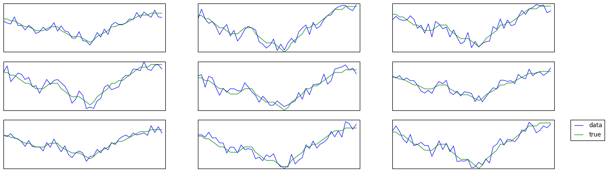
学習データX（各時刻における特徴）とy（真の固定時系列）を確認のため比較．

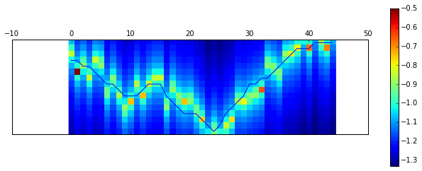
確認

plt.matshow(np.flipud(X_train[0,:,:-1].T)) # remove bias
plt.colorbar()
plt.yticks(())
#plt.show()

plt.plot(15-y_train[0]) # flipud
plt.show()

では学習器の準備．
PyStructのChainCRFの説明にしたがって，FrancWolfeSSVMで学習．

学習器の準備

from pystruct.models import ChainCRF
from pystruct.learners import FrankWolfeSSVM
model = ChainCRF()
ssvm = FrankWolfeSSVM(model=model, C=.1, max_iter=10)

学習！

%%time
ssvm.fit(X_train, y_train)
====
CPU times: user 1.25 s, sys: 17.4 ms, total: 1.27 s
Wall time: 1.3 s

FrankWolfeSSVM(C=0.1, batch_mode=False, check_dual_every=10,
        do_averaging=True, line_search=True, logger=None, max_iter=10,
        model=ChainCRF(n_states: 16, inference_method: max-product),
        n_jobs=1, random_state=None, sample_method='perm',
        show_loss_every=0, tol=0.001, verbose=0)

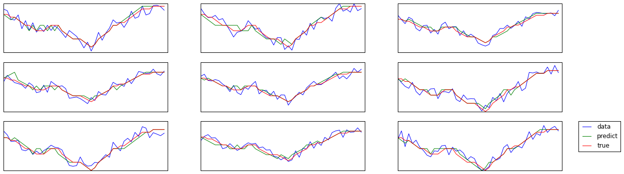
それでは予測スコアは？

ssvm.score(X_test, y_test)
==========
0.56377777777777771

テストに対する予測を確認

X_test_predict = np.array(ssvm.predict(X_test))

fig, axes = plt.subplots(3,3, figsize=(20,6))
shf = np.arange(X_test.shape[0])
np.random.shuffle(shf)
c=0
for ax in axes.ravel():
    ax.plot(data[shf[c]], label='data')
    ax.plot(X_test_predict[shf[c]], label='predict')
    ax.plot(y_test[shf[c]], label='true')
    ax.set_xticks(())
    ax.set_yticks(())
    c += 1

plt.legend(bbox_to_anchor=(1.1, 1.0), loc=2, borderaxespad=0.)

学習されたwを確認

ssvm.w.shape # = n_features * n_states + n_states**2
========
(528,)

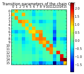
ペアワイズの重みw

plt.matshow(ssvm.w[n_features * n_states:].reshape(n_states, n_states))
plt.title("Transition parameters of the chain CRF.")
plt.xticks(np.arange(n_states))
plt.yticks(np.arange(n_states))
plt.colorbar()
plt.show()

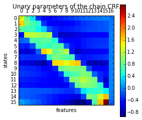
unaryの重みw

plt.matshow(ssvm.w[:n_features * n_states].reshape(n_states,n_features))
plt.title("Unary parameters of the chain CRF.")
plt.yticks(np.arange(n_states))
plt.xticks(np.arange(n_features))
plt.ylabel('states') 
plt.xlabel('features')
plt.colorbar()
plt.show()