この記事に載せているX Learnerのコードは書き方に無駄が多く変数の名づけも適当で綺麗でないのでClassにしました。
因果推論 Uplift Modeling X Learner for Multiple Treatments【Python】
はじめに
この記事は、Uplift Modeling for Multiple Treatments with Cost Optimization の内容をベースとしています。

先ずはこの記事の構成を示します。
- 論文の紹介 (Uplift Modeling for Multiple Treatments with Cost Optimization)
- X-Learner と Extending X-learner for Multiple Treatments のアルゴリズム (X-Learner & Extending X-Learner for Multiple Treatments)
- Extending X-learner for Multiple Treatments の実装 (Implementation)
- Extending X-learner for Multiple Treatments にチャンネル、想定されるコンバージョン、施策によるコンバージョン、施策コスト、CPM課金の要素を組み込んだアルゴリズム (Extending X-Learner for Net Value CATE)
- まとめ (まとめ)
- 参考 URL (参考URL)
この記事では因果推論の考え方や Uplift Modeling (因果推論と機械学習の関係) について解説はしていませんがこの記事を書くにあたり参考になった論文やサイトを 参考 URL として載せてあります。
Uplift Modeling for Multiple Treatments with Cost Optimization
Uber Eats を運営する Uber (Uber Technologies Inc.) からとても興味深い内容の論文が発表されています。
論文にはそのモチベーションが以下のように書かれています。
There are a few existing uplift modeling methods proposed for multiple treatment groups, however, there are sparse existing implementations of the state-ofthe-art algorithms in the multi-treatment context to support industry applications. It also leads to little evidence as to which algorithms in fact are state-of-the-art in the multi-arm context in practice in terms of model accuracy and computation performance. In this paper we aim to bridge this gap by extending two meta-learner models originally designed for one treatment and one control case to multiple
treatment group case, and then ...
(Uplift Modeling for Multiple Treatments with Cost Optimization)
概要はその説明をされている note から抜粋します。
Uberは複数の施策を顧客に行ったときに、どの施策が最もコストパフォーマンスが良いかをX-Learner,R-Learnerを改良した方法を用いて検証しています。
Uplift modelingの手法を用いて、どの顧客にどんなチャネルでどのようなキャンペーンを打てばコストパフォーマンスが良いかを検証します。また、キャンペーン以外にも、アプリ内のデザイン・コンテンツ、その他変更可能な部分を戦略的にパーソナライズでき、誰に何をどのように提供すべきかが明確になります。
(Uber徹底研究 -因果推論によるマーケティング最適化編-)
X-Learner & Extending X-Learner for Multiple Treatments
X-Learner と Extending X-Learner for Multiple Treatments それぞれのアルゴリズムを紹介します。
X-Learner の考え方は 2 つの段階に分けられます。
1 段階目では Treatment / Control それぞれの効果 $\mu_{1}, \ \mu_{0}$ を推定。
2 段階目では既に推定された効果と結果変数の差分を利用し条件付き期待値を算出。さらに傾向スコアで重みづけをすることで精度を高めています。
CATE の推定において「CATE がスパースな場合」「CATE の滑らかさ」「Treatment / Control 群の間に偏りがある場合」に対しある程度の対応をすることができます。
Extending X-Learner for Multiple Treatments は X-Learner を拡張し複数介入のケースにも対応できるようにした Meta-Learner のアルゴリズムです。
これはつまり「X-Learner は $t_j ∈ \{t_0, t_1\}$ を考えている」のに対し「Extending X-Learner for Multiple Treatments は $t_j ∈ \{t_0, t_1, ..., t_m\} \ (j ∈ \mathbb{Z})$ を考えている」ということを意味しています。
数式からも見て取れるように考え方の流れは X-Learner と同じです。
Extending X-Learner for Multiple Treatments をさらに拡張した Extending X-Learner for Net Value CATE のアルゴリズムを実装の後に紹介しています。
(Extending X-Learner for Net Value CATE)
X-Learner
“pseudo-effects” ${D_{i}}$ for the observations in the control group as
\tilde{D_{i}^{0}} = \widehat{\mu }_{1}\left( x\right) - Y_{i}^{0} \tag{1}
and for the individuals in the treatment groups as
\tilde{D_{i}^{1}} = Y_{i}^{1} - \widehat{\mu }_{0}\left( x\right) \tag{2}
where ${Y_{i}}$ is the observed value for the user. The pseudo-effects are then used as the outcome in another pair of regression methods to obtain the response functions ${\tilde{\tau_{1}^{}}(x)}$ and ${\tilde{\tau_{1}^{}}(x)}$ for the control and treatment groups, respectively.
\begin{aligned}\widehat{\tau }\left( x\right) =e\left( x\right) \widehat{\tau }_{0}\left( x\right) +\left( 1-e\left( x\right) \right) \widehat{\tau }_{1}\left( x\right) \end{aligned} \tag{3}
where ${e(x)}$ is the propensity score $P[W_{i} = 1 \ | \ X_{i} = x]$ with ${W_{i}}$ indicating the treatment assignment.
Extending X-Learner for Multiple Treatments
Consider an experiment with a control group and m treatment groups. Here, we use any suitable regression method to estimate the response functions under each group:
\begin{aligned}\mu _{t_{j}}\left( x\right) = \mathbb{E}[ Y\left( t_{j}\right) \ | \ X=x] \end{aligned} \tag{4}
where $t_j ∈ \{t_0, t_1, ..., t_m\}$ with t0 denoting the control group.
We estimate ${\mu_{t_{0}}(x)}$ using data from the control group and${\mu_{t_{1}}(x)}$ using data from the j-th treatment group. We then proceed to estimate the pseudo-effects analogously,
{\begin{equation}
  \begin{split}
\tilde{D_{i}^{t_{0}}} = \hat{\mu} _{t_{j}}(x) - Y_{i}
\\
\tilde{D_{i}^{t_{j}}} = Y_{i} - \hat{\mu} _{t_{0}}(x)
  \end{split}
\end{equation}
} \tag{5}
where ${\tilde{D_{i}^{t_{0}}}}$ is estimated using control group data and ${\tilde{D_{i}^{t_{j}}}}$ is estimated using the data from the j-th treatment group. Finally, as in the two-group experiment, we use the pseudo-effects as
the outcomes in another pair of regressions to obtain $\hat{\tau} _{t_0}$ and $\hat{\tau}_{t_j}$.
In the multiple treatment group case, we need to estimate
the propensity score
e_{t_{j}}(x) \ = \ \mathbb{P}[W_{i} = t_{j} \ | \ X = x] \tag{6}
for each m experiment groups. Focusing on the case in which we compare each treatment group against the control, we then estimate the CATEor a given treatment group as follows :
\hat{\tau}^{t_{j}}(x) = \dfrac{\hat{e}_{t_j}(x)}{\hat{e}_{t_j}(x) + \hat{e}_{t_0}(x)}\hat{\tau}_{t_0}(x) \ + \ \dfrac{\hat{e}_{t_0}(x)}{\hat{e}_{t_j}(x) + \hat{e}_{t_0}(x)}\hat{\tau}_{t_j}(x) \tag{7}
Finally, to predict the best treatment group for an individual,
we estimate $\tau^{t_j}$ as
\hat{\tau}^{t_{j}}(X_i) = \dfrac{\hat{e}_{t_j}^{(-1)}(X_i)}{\hat{e}_{t_j}^{(-1)}(X_i) + \hat{e}_{t_0}^{(-1)}(X_i)}\hat{\tau}_{t_0}^{(-1)}(X_i) + \dfrac{\hat{e}_{t_0}^{(-1)}(X_i)}{\hat{e}_{t_j}^{(-1)}(X_i) + \hat{e}_{t_0}^{(-1)}(X_i)}\hat{\tau}_{t_j}^{(-1)}(X_i) \tag{8}
where notation of the form $\hat{e} _{t_j}^{(-1)}$ indicates that $\hat{e}_{t_j}$ has been estimated without using the $i$-th observation. We then simply compare which treatment group gives the highest predicted uplift for the individual and recommend that as the treatment group if the costs of treatments are equal.
実装
X-Learner for Multiple Treatments を実装していきます。
<必要なライブラリの読み込み>
import pandas as pd
import numpy as np
import matplotlib.pyplot as plt
%matplotlib inline
from copy import deepcopy

from sklearn.model_selection import KFold
from sklearn.metrics import mean_squared_error as mse
from sklearn.metrics import log_loss

from causalml.dataset import synthetic_data, get_synthetic_summary_holdout
from causalml.propensity import compute_propensity_score
from causalml.metrics import plot, auuc_score
from causalml.inference.meta import BaseXRegressor

from sklearn.linear_model import LogisticRegression
from sklearn.ensemble import RandomForestClassifier
import lightgbm as lgb
<利用するデータの生成>
y : コンバージョン (結果変数)
X : 共変量
treatment : 介入の種類(生成されるデータは「介入なし : 0 または 介入あり : 1」の 2 値ですが今回は簡単のためにこのデータを用いています。)
e : 傾向スコア(生成されるデータは $e(x) = P[treatment = 1 \ | \ X = x]$ であるためこのデータは用いていません。)
y, X, treatment, _, _, e = synthetic_data(mode = 1, n = 10000, p = 5, sigma = 1.0)

synthetic_data_ = np.hstack(( y.reshape(len(y), 1), X, treatment.reshape(len(y), 1), e.reshape(len(y), 1) ))
synthetic_df = pd.DataFrame(data = synthetic_data_)
synthetic_df.rename(columns = {0 : 'Y', 1 : 'cova_1', 2 : 'cova_2',
                               3 : 'cova_3', 4 : 'cova_4', 5 : 'cova_5',
                               6 : 'inte', 7 :  'ps'}, inplace = True)
<傾向スコアの算出>
「X-Learner」と比較して「Extending X-Learner for Multiple Treatments」ではそれぞれの介入に対応する傾向スコアをCATEの算出に用います。
X-Learner : $e(x) = P[W_{i} = 1 \ | \ X_{i} = x]$ with $W_{i}$ indicating the treatment assignment
Extending X-Learner for Multiple Treatments : $e_{t_{j}}(x) \ = \ \mathbb{P}[W_{i} = t_{j} \ | \ X = x]$ for each m experiment groups
今回は簡単のために 単一介入( np.unique(treatment) = [0, 1] )のデータを用いていますが以下のコードは 複数介入( np.unique(treatment) = [0, 1, ..., n] ) のデータにも対応させたものです。
def propensity_score_RF(X, z, n_splits):
    if type(X) == np.ndarray or type(z) == np.ndarray:
        X = pd.DataFrame(data = X)
        z = pd.DataFrame(data = z)

    groups = z.unique()
    num_groups = len(groups)

    for i in range(num_groups):
        preds_rf = {i: np.zeros(X.shape[0]) for i in range(num_groups)}
        logloss_rf_train = {i: [] for i in range(num_groups)}
        logloss_rf_valid = {i: [] for i in range(num_groups)}

    kf = KFold(n_splits = n_splits, shuffle = True, random_state = 0)
    for n_fold, (train_index, valid_index) in enumerate(kf.split(X)):
        print('CV_{}'.format(n_fold))
        X_train, z_train = X.iloc[train_index], z.iloc[train_index]
        X_valid, z_valid = X.iloc[valid_index], z.iloc[valid_index]

        print('RandomForestClassifier_progressing...')
        model_rf = RandomForestClassifier()
        model_rf.fit(X_train, z_train)

        pred_proba_train = {i : model_rf.predict_proba(X_train)[:, i] for i in range(num_groups) }
        logloss_train = { i : log_loss(z_train, pred_proba_train[i]) for i in range(num_groups) }
        for i in range(num_groups):
            logloss_rf_train[i].append(logloss_train[i])

        pred_proba_valid = { i : model_rf.predict_proba(X_valid)[:, i] for i in range(num_groups) }
        for i in range(num_groups):
            preds_rf[i][valid_index] = pred_proba_valid[i]

        logloss_valid = { i : log_loss(z_valid, pred_proba_valid[i]) for i in range(num_groups)}
        for i in range(num_groups):
            logloss_rf_valid[i].append(logloss_valid[i])

    logloss_rf_train_ = { i : sum(logloss_rf_train[i]) / n_splits for i in range(num_groups) }
    logloss_rf_valid_ = { i : sum(logloss_rf_valid[i]) / n_splits for i in range(num_groups) }

    eps = np.finfo(float).eps
    preds_rf = { i : np.where(preds_rf[i] < 0 + eps, 0 + eps*1.001, preds_rf[i]) for i in range(num_groups) }
    preds_rf = { i : np.where(preds_rf[i] > 1 - eps, 1 - eps*1.001, preds_rf[i]) for i in range(num_groups) }

    print('Complete')

    return preds_rf, logloss_rf_train_, logloss_rf_valid_

ps, logloss_rf_train, logloss_rf_valid = propensity_score_RF(X = X, z = z, n_splits = 5)
<条件付き平均処置効果(CATE)の推定>
def fit_predict(data, X_col, intervention_col, y_col, ps_col, verbose = True):
    if control_outcome_learner is None:
        model_mu_c = deepcopy(learner)
    else:
        model_mu_c = control_outcome_learner

    if treatment_outcome_learner is None:
        model_mu_t = deepcopy(learner)
    else:
        model_mu_t = treatment_outcome_learner

    if control_effect_learner is None:
        model_tau_c = deepcopy(learner)
    else:
        model_tau_c = control_effect_learner

    if treatment_effect_learner is None:
        model_tau_t = deepcopy(learner)
    else:
        model_tau_t = treatment_effect_learner

    tmp = data
    control_name = 0
    t_groups = np.unique(tmp[intervention_col].loc[tmp[intervention_col] != control_name])
    t_groups.sort()
    _classes = {group: i for i, group in enumerate(t_groups)}

    num_ps_col = len(ps_col)
    ps_col_ = { i : ps_col[i] for i in range(num_ps_col) }
    ps_ = { i : np.array(tmp[ps_col_[i]]) for i in range(num_ps_col) }

    te = np.zeros((X.shape[0], t_groups.shape[0]))
    dhat_cs = {}
    dhat_ts = {}

    for group in t_groups:
        models_mu_c = {group: deepcopy(model_mu_c) for group in t_groups}
        models_mu_t = {group: deepcopy(model_mu_t) for group in t_groups}
        models_tau_c = {group: deepcopy(model_tau_c) for group in t_groups}
        models_tau_t = {group: deepcopy(model_tau_t) for group in t_groups}

        models_mu_c[group].fit(tmp.loc[tmp[intervention_col] == 0, X_col], tmp.loc[tmp[intervention_col] == 0, y_col])
        models_mu_t[group].fit(tmp.loc[tmp[intervention_col] == group, X_col], tmp.loc[tmp[intervention_col] == group, y_col])

        d_c = models_mu_t[group].predict(tmp.loc[tmp[intervention_col] == 0, X_col]) - tmp.loc[tmp[intervention_col] == 0, y_col]
        d_t = tmp.loc[tmp[intervention_col] == group, y_col] - models_mu_c[group].predict(tmp.loc[tmp[intervention_col] == group, X_col])

        models_tau_c[group].fit(tmp.loc[tmp[intervention_col] == 0, X_col], d_c)
        models_tau_t[group].fit(tmp.loc[tmp[intervention_col] == group, X_col], d_t)

        dhat_cs[group] = models_tau_c[group].predict(tmp[X_col])
        dhat_ts[group] = models_tau_t[group].predict(tmp[X_col])

        te_ = ((ps_[group] / (ps_[group] + ps_[0])) *  dhat_cs[group] + (ps_[0] / (ps_[group] + ps_[0])) * dhat_ts[group]).reshape(-1, 1)
        group_ = int(group) - 1
        te[:, group_] = np.ravel(te_)

    if verbose:
        for group in t_groups:
            print('Treatment group : {}'.format(int(group)))

            # RMSE for verbose
            y_hat_control = models_mu_c[group].predict(tmp.loc[tmp[intervention_col] == 0, X_col])
            y_hat_treatment = models_mu_t[group].predict(tmp.loc[tmp[intervention_col] == group, X_col])

            rmse_ = np.sqrt(mse(np.array(tmp.loc[tmp[intervention_col] == 0, y_col]), np.array(y_hat_control)))
            print('RMSE   (Control): %s' %rmse_)
            rmse_ = np.sqrt(mse(np.array(tmp.loc[tmp[intervention_col] == group, y_col]), np.array(y_hat_treatment)))
            print('RMSE (Treatment): %s' %rmse_)

            # Gini Coefficient for verbose
            arr_control = np.array([np.array(tmp.loc[tmp[intervention_col] == 0, y_col]), y_hat_control]).transpose()
            arr_treatment = np.array([np.array(tmp.loc[tmp[intervention_col] == group, y_col]), y_hat_treatment]).transpose()

            for i, arr in enumerate([arr_control, arr_treatment]):
                if i == 0:
                    n_samples = tmp.loc[tmp[intervention_col] == 0, y_col].shape[0]
                elif i == 1:
                    n_samples = tmp.loc[tmp[intervention_col] == group, y_col].shape[0]

                # sort rows on prediction column
                # (from largest to smallest)
                true_order = arr[arr[:, 0].argsort()][::-1, 0]
                pred_order = arr[arr[:, 1].argsort()][::-1, 0]

                # get Lorenz curves
                l_true = np.cumsum(true_order) / np.sum(true_order)
                l_pred = np.cumsum(pred_order) / np.sum(pred_order)
                l_ones = np.linspace(1 / n_samples, 1, n_samples)

                # get Gini coefficients (area between curves)
                g_true = np.sum(l_ones - l_true)
                g_pred = np.sum(l_ones - l_pred)

                # normalize to true Gini coefficient
                true_gini = g_pred / g_true

                if i == 0:
                    print('Gini   (Control): %s' %true_gini)
                elif i == 1:
                    print('Gini (Treatment): %s' %true_gini)

    return te


# learner (optional): a model to estimate outcomes and treatment effects in both the control and treatment groups
# control_outcome_learner (optional): a model to estimate outcomes in the control group
# treatment_outcome_learner (optional): a model to estimate outcomes in the treatment group
# control_effect_learner (optional): a model to estimate treatment effects in the control group
# treatment_effect_learner (optional): a model to estimate treatment effects in the treatment group

learner = lgb.LGBMRegressor(boosting_type = 'gbdt', objective = 'regression', reg_alpha = 1, reg_lambda = 1,
                            subsample = 0.6, max_depth = 10, num_leaves = 20,
                            colsample_bytree = 0.5, min_child_weight = 10,
                            n_estimators = 1000)
control_outcome_learner = None
treatment_outcome_learner = None
control_effect_learner = None
treatment_effect_learner = None

synthetic_df['ps_0'] = ps[0]
synthetic_df['ps_1'] = ps[1]

data = synthetic_df
X_col = X_col = ['cova_1', 'cova_2', 'cova_3', 'cova_4', 'cova_5']
y_col = 'Y'
intervention_col = 'inte'
ps_col = ['ps_0', 'ps_1']

cate = fit_predict(data, X_col, intervention_col, y_col, ps_col, verbose = True)
<causalmlとの比較>
この実装では単一介入( np.unique(treatment) = [0, 1] )のデータから CATE を算出しているため causalml を用いて CATE を算出することもできます。
learner_x = BaseXRegressor(learner = learner)
cate_x = learner_x.fit_predict(X = X, treatment = treatment, y = synthetic_df['Y'], p = e, return_ci = False)
alpha = 0.2
bins = 30
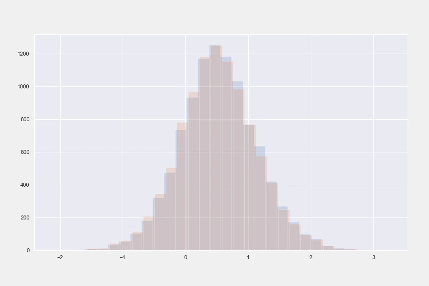
plt.figure(figsize = (12, 8))
plt.hist(cate_x, alpha = alpha, bins = bins, label = 'X Learner')
plt.hist(cate, alpha = alpha, bins = bins, label = 'X Learner Multiple')
plt.legend()
plt.show()
Extending X-learner for Multiple Treatments (red) VS causalml (blue)
<モデルの評価>
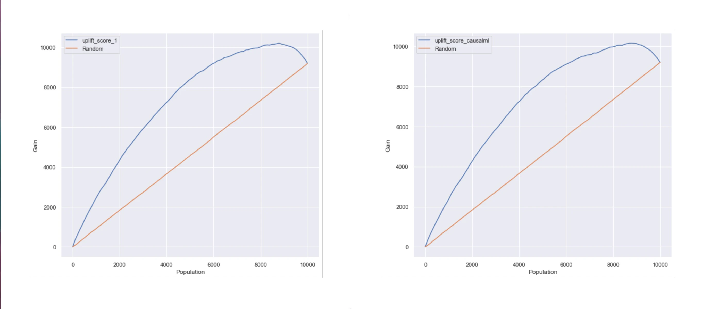
AUUC (Area Under the Uplift Curve)からモデルの評価を行います。
lift : 適当なスコアをしきい値として「しきい値以上の対象にのみ介入を行った場合の CV 」が「介入を全く行わなかった場合の CV」と比較してどれだけ上昇しているかの値。
baseline : 適当なスコアをしきい値として「しきい値以上の対象にのみランダムに介入を行った場合の CV 」が「介入を全く行わなかった場合の CV」と比較してどれだけ上昇しているかの値。ランダムな介入は観測できないため lift 曲線の左端と右端を結んだ直線を baseline とする。
グラフの横軸は Uplift Score (CATE) の降順を表し lift 曲線よりも下のエリアの面積が AUUC(介入を行わなかった場合と比較した CV の上昇数) を表します。
AUUC の値が大きいほどモデルから算出された施策の効果はあると評価できます。
accu_score_ = auuc_score(df = synthetic_df[['Y','inte', 'uplift_score_1']], kind = 'gain',
                        outcome_col = 'Y',
                        treatment_col = 'inte')
print('AUUC : %s' %accu_score_)

threshold = synthetic_df['uplift_score_1'].sort_values(ascending = False).reset_index(drop = True)[8700]
print('Threshold : %s' %threshold)


plot(df = synthetic_df[['Y','inte', 'uplift_score_1']], kind = 'gain',
     outcome_col = 'Y',
     treatment_col = 'inte'
    )
plot(df = synthetic_df[['Y','inte', 'uplift_score_causalml']], kind = 'gain',
     outcome_col = 'Y',
     treatment_col = 'inte'
    )
AUUC : uplift_score_1    0.788084
Random            0.498509
dtype: float64
Threshold : -0.1383321462934351
Extending X-learner for Multiple Treatments (left) VS causalml (right)
Net Value Optimization for Multiple Treatment Groups with Different Costs
Extending X-learner for Multiple Treatments にチャンネル、想定されるコンバージョン、施策によるコンバージョン、施策コスト、CPM課金の要素を組み込んだアルゴリズムを紹介します。
AUUC による検証において Net Value X-Learner は X-Learner や R-learner など従来のモデルと比較して 2 倍のパフォーマンスを発揮しています。
Extending X-Learner for Net Value CATE
Extending X-Learner for Net Value CATE
This section proposes Modified models that estimate and optimize the net value uplift in a multi-arm context.
The following notations are used for formulating the value and cost structure :
• $v$: conversion value, assuming each conversion is weighted equally and the conversion value is a constant given as prior knowledge.
• $c_{t_j} \ for \ j \ ∈ \ \{0, 1, 2, .., m\}$: impression cost for each treatment paid for each treated user, for example, the channel cost per send.
• $s_{t_j} \ for \ j \ ∈\ \{0, 1, 2, .., m\}$: triggered cost for each
treatment paid for each converted user, for example, the
promotion code applied by the user for purchase.
The expected net value for user $i$ under treatment ${t_{j}}$ can be defined as $E[(v − s_{t_j})Y_{t_j} − c_{t_j} \ | \ X = x]$.
Extending X-Learner for Net Value CATE: To modify the X-Learner for estimating the net value CATE, we keep most part of the formulation unchanged, including the base models for estimating the outcome (4), propensity score model (6), as well as the final CATE estimation equation (8). The main modification happens to the pseudo-effects (5). Instead of constructing the pseudo-effects on the original outcome variable $Y$ , the modified X-Learner formulates the net value pseudo-effects as:
\begin{equation}
  \begin{split}
\tilde{D}_{i}^{t_j, t_0}(x_{i}^{t_j}, Y_{i}^{t_j}) = (v -s_{t_j})Y_{i}^{t_j} - (v - s_{t_0})\mu_{t_0}(x_{i}^{t_j}) - (c_{t_j} - c_{t_0})
\\
\tilde{D}_{i}^{t_j, t_0}(x_{i}^{t_0}, Y_{i}^{t_0}) = (v -s_{t_j})\mu_{t_j}(x_{i}^{t_0})- (v - s_{t_0})Y_{i}^{t_0} - (c_{t_j} - c_{t_0})
  \end{split}
\end{equation} \tag{9}
where notation of the form ${x_{i}^{t_j}}$ indicates we have used the observations form the ${j}$-th treatment group.
A standard regression model can be fit on the net value
pseudo-effects, and the corresponding estimator is denoted as ${\hat{\tau} _{t_j}(x)}$ for treatment ${\tau_{j}}$. The rest of the algorithm follows the same as the X-Learner for multiple treatments.
まとめ
Uplift Modeling for Multiple Treatments with Cost Optimization の内容をもとに Extending X-Learner for Multiple Treatments を実装してみました。
コードに関しての間違いなどありましたらご指摘のほどよろしくお願いいたします。
参考 URL
<論文>
Uplift Modeling for Multiple Treatments with Cost Optimization (Zhenyu Zhao, Totte Harinen)
Quasi-Oracle Estimation of Heterogeneous Treatment Effects (Xinkun Nie, Stefan Wager)
Counterfactual Cross-Validation: Stable Model Selection Procedure for Causal Inference Models (Yuta Saito, Shota Yasui)
<書籍>
(効果検証入門~正しい比較のための因果推論/計量経済学の基礎~ 著者: 安井 翔太 / 出版: 技術評論社 / 発売日: 2020/01/18)
計量経済学における因果推論の基礎を学ぶにはうってつけな一冊だと思います。
こちらの本では軽量経済学においての Rubin の因果推論について順序だてて丁寧な解説がされておりその内容には CausalImpact についての解説もあります。
統計的因果推論を行う上でその土台となる実験デザインについてもしっかりと説明がなされている本はとても魅力的ではないでしょうか。
<サイト>
AIで原因と結果を把握する ~機械学習と因果推論の融合 Meta-Learner~
ノーベル経済学賞でも注目の因果推論を俯瞰する
Uber徹底研究 -因果推論によるマーケティング最適化編-
傾向スコアを用いた因果推論入門~理論編~
傾向スコアを用いた因果推論入門~実装編~