多項式回帰で重回帰分析やってみた

単回帰と重回帰

• 単回帰…一つの入力データを使って、ある値を予測しようとする手法。

ex)身長のデータを使って体重を予測。
y=w₀+w₁X

• 重回帰…二つ以上の入力データを使って、ある値を予測しようとする手法。

ex)身長、ウエスト、体脂肪…を使って、体重を予測。
y=w₀+w₁x₁+w₂x₂+w₃x₃+…

多項式回帰による例

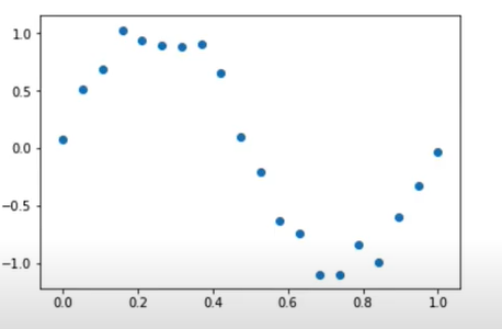
• 今、下図のようなデータを回帰したい。しかし、明らかに直線では表現できない形だ。

• 多項式回帰によって回帰を試みる。

• 多項式回帰…重回帰分析の一種。入力データxに加えてx^2,x^3…を新たな入力データとして加える。

最小二乗法は万能ではない

• 最小二乗法はモデルが複雑化しやすいアルゴリズム。

学習不足・過学習という問題

• 学習不足…訓練データを十分に表現できていない状況。損失関数が高いまま。

• 過学習(過剰適合)…訓練データに過度に適合している状況。汎化性能が低くなっている。

正則化というテクニック

• 正則化…適切な係数を取捨選択したり、係数の大きさを小さくして、過学習を防止する手法。本当に大切な係数を見つけ出す。

• 変数選択
  漸次的選択法…係数を一つずつ足す、もしくは減らしながら当てはまりの良さを最大にしていく。

• 縮小推定
  ①リッジ回帰…係数の絶対値を縮小する。
  ②Lasso回帰…いくつかの係数を完全に0にする。

実践(多項式回帰)

import numpy as np
import matplotlib.pyplot as plt

data_size=20
#0~1までを20個区切りで表す。
X=np.linspace(0,1,data_size)

#low以上high未満の一様乱数
noise=np.random.uniform(low=-1.0,high=1.0,size=data_size)*0.2

y=np.sin(2.0*np.pi*X)+noise

#0~1までを1000個区切りで表す。
X_line=np.linspace(0,1,1000)
sin_X=np.sin(2.0*np.pi*X_line)

def plot_sin():
    plt.scatter(X,y)
    plt.plot(X_line,sin_X,"red")
plot_sin()

from sklearn.linear_model import LinearRegression

#線形回帰モデル生成
lin_reg_model=LinearRegression().fit(X.reshape(-1,1),y)

#切片,傾き
lin_reg_model.intercept_,lin_reg_model.coef_

plt.plot(X_line,lin_reg_model.intercept_+lin_reg_model.coef_*X_line)
plot_sin()

from sklearn.preprocessing import PolynomialFeatures

#0乗~3乗までの4つのカラムを生成(20行4列のデータフレーム生成)
poly = PolynomialFeatures(degree=3)
poly.fit(X.reshape(-1,1))
X_poly_3=poly.transform(X.reshape(-1,1))

lin_reg_3_model=LinearRegression().fit(X_poly_3,y)

X_line_poly_3=poly.fit_transform(X_line.reshape(-1,1))
plt.plot(X_line,lin_reg_3_model.predict(X_line_poly_3))
plot_sin()

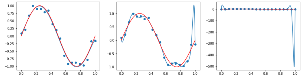
fig,axes=plt.subplots(1,3,figsize=(16,4))

for degree,ax in zip([5,15,25],axes):
    poly=PolynomialFeatures(degree=degree)
    X_poly=poly.fit_transform(X.reshape(-1,1))
    lin_reg=LinearRegression().fit(X_poly,y)
    X_line_poly=poly.fit_transform(X_line.reshape(-1,1))
    ax.plot(X_line,lin_reg.predict(X_line_poly))
    ax.scatter(X,y)
    ax.plot(X_line,sin_X,"red")

実践(正規化)

import mglearn
import pandas as pd
from sklearn.model_selection import  train_test_split

X,y=mglearn.datasets.load_extended_boston()
df_X=pd.DataFrame(X)
dy_y=pd.DataFrame(y)

X_train,X_test,y_train,y_test=train_test_split(X,y,random_state=0)

lin_reg_model=LinearRegression().fit(X_train,y_train)

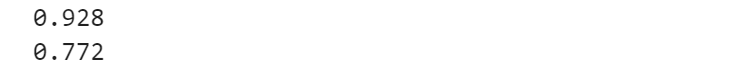
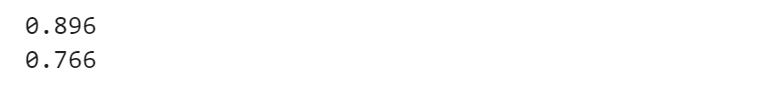
print(round(lin_reg_model.score(X_train,y_train),3))#訓練データ適合率
print(round(lin_reg_model.score(X_test,y_test),3))#テストデータ適合率

リッジ回帰モデル生成

from sklearn.linear_model import Ridge,Lasso

ridge_model=Ridge().fit(X_train,y_train)

def print_score(model):
    print(round(model.score(X_train,y_train),3))#訓練データ適合率
    print(round(model.score(X_test,y_test),3))#テストデータ適合率

#alphaが大きいほど絶対値を小さく(default=1)
ridge_10_model=Ridge(alpha=10).fit(X_train,y_train)
print_score(ridge_10_model)

ridge_01_model=Ridge(alpha=0.1).fit(X_train,y_train)
print_score(ridge_01_model)

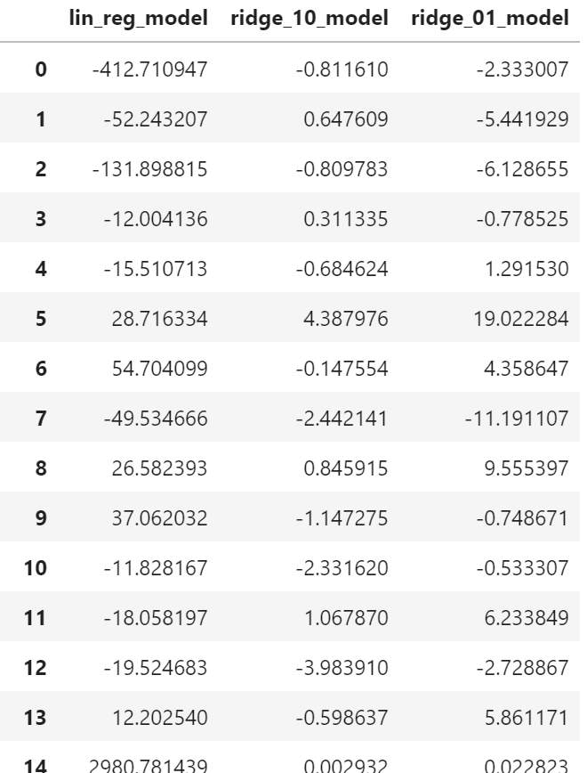
coefficients=pd.DataFrame({"lin_reg":lin_reg.coef_,"ridge_10_model":ridge_10_model.coef_,"ridge_01_model":ridge_01_model.coef_})
coefficients

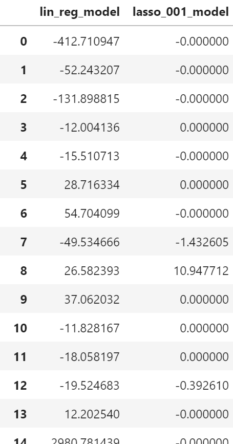
Lasso回帰モデル生成

lasso_001_model=Lasso(alpha=0.01,max_iter=10000).fit(X_train,y_train)
print_score(lasso_001_model)

coefficients_lasso=pd.DataFrame({"lin_reg":lin_reg.coef_,

                                 "lasso_001_model":lasso_001_model.coef_})