キノコの毒の有無を予測する

1.はじめに

こんにちは、tomoです。

ここ2ヶ月間、データサイエンスの基礎理論について、学習サイトや書籍で学んできました。
（Aidemy「Matplotlibによるデータの可視化」、書籍「python 機械学習プログラミング」など。）

理解できていない箇所の洗い出し、また、実践力を鍛えることを目的に、データ分析記事を投稿します。

2.分析対象を探す

オープンデータで面白そうなデータがないか探します。
例えば以下のサイト。

UC Irvine Machine Learning Repository

一際異彩を放つデータを見つけました。

Mushroom

コレ、勇ましくそびえ立っているのにビビっと来たので、このデータを分析します。

3.データの概要を掴む

Mushroomの説明欄を読みます。
　「Data Set Information」・・・データセットの概要
　「Attribute Information」・・・データセットに含まれる特徴の説明

どうやら各データには「食べられる」、「毒がある（＝食べられない）」の情報と、その判別の補助となる情報（かさの色、生息地など）が含まれているようです。

今回はキノコに毒があるかどうかを予測するモデルを構築します。

4.モデルの構築

それではデータをいじっていきます。
まずはデータダウンロードし、読み込みます。

import pandas as pd

#mushroomのデータを読み込む
mr_data = pd.read_csv('ダウンロードしたデータのパス')

#列名を設定
mr_data.columns = ["edibility","cap-shape","cap-surface","cap-color","bruises","odor","gill-attachment","gill-spacing","gill-size","gill-color","stalk-shape","stalk-root","stalk-surface-above-ring","stalk-surface-below-ring","stalk-color-above-ring","stalk-color-below-ring","veil-type","veil-color","ring-number","ring-type","spore-print-color","population","habitat"]

データの読み込みが完了したら、中身を確認します。

#データの内容を確認
mr_data.head()

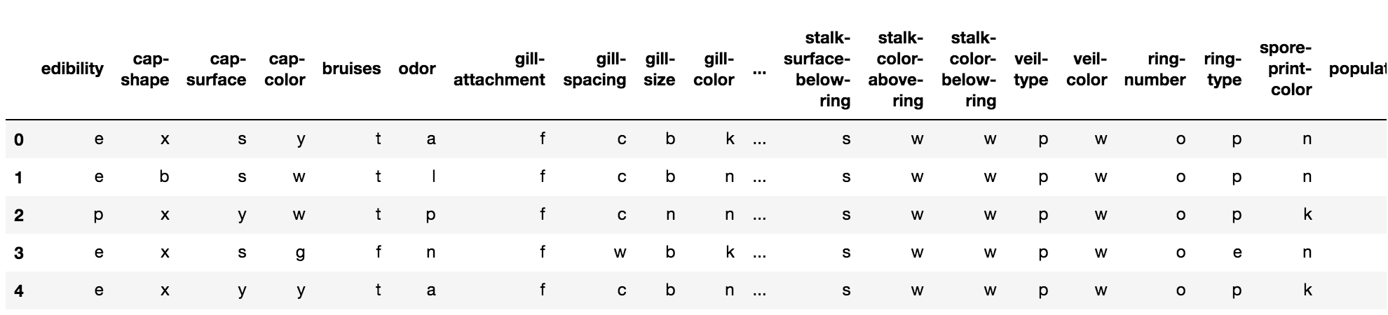
無事読み込めています。「Attribute Information」の説明の通り、英字1文字のデータが並んでいます。
データに欠損値が無いか確認します。

#欠損値の数を数える
mr_data.isnull().sum()

edibility                   0
cap-shape                   0
cap-surface                 0
cap-color                   0
bruises                     0
odor                        0
gill-attachment             0
gill-spacing                0
gill-size                   0
gill-color                  0
stalk-shape                 0
stalk-root                  0
stalk-surface-above-ring    0
stalk-surface-below-ring    0
stalk-color-above-ring      0
stalk-color-below-ring      0
veil-type                   0
veil-color                  0
ring-number                 0
ring-type                   0
spore-print-color           0
population                  0
habitat                     0

欠損値は無いようです。欠損値が見つかった場合、平均や中央値などで補完したり、また、欠損値があまりに多い特徴は丸ごと削除するなど、対応が必要になります。

続いて、データの変数化を実施します。
順序関係が無い特徴についてはダミー変数化しますが、順序性がある特徴はカテゴリ変数化します。
（ただし、ダミー変数については多重共線性に気をつける必要があります。）

まずはダミー変数化から。

#順序関係が含まれないクラスをダミー変数化
mr_data_le = pd.get_dummies(mr_data, drop_first=True, columns=["cap-shape","cap-surface","cap-color","bruises","odor","gill-attachment","gill-color","stalk-shape","stalk-root","stalk-surface-above-ring","stalk-surface-below-ring","stalk-color-above-ring","stalk-color-below-ring","veil-type","veil-color","ring-type","spore-print-color","habitat"])

続いて順序関係が含まれる特徴について、カテゴリ変数化を実施。

from sklearn import preprocessing

#順序関係が含まれるクラスをカテゴリ変数化
for column in ["edibility","gill-spacing","gill-size","ring-number","population"]:
    selected_column = mr_data_le[column]
    le = preprocessing.LabelEncoder()
    le.fit(selected_column)
    column_le = le.transform(selected_column)
    mr_data_le[column] = pd.Series(column_le).astype('category')

データの中身を再度確認します。

mr_data_le.head()

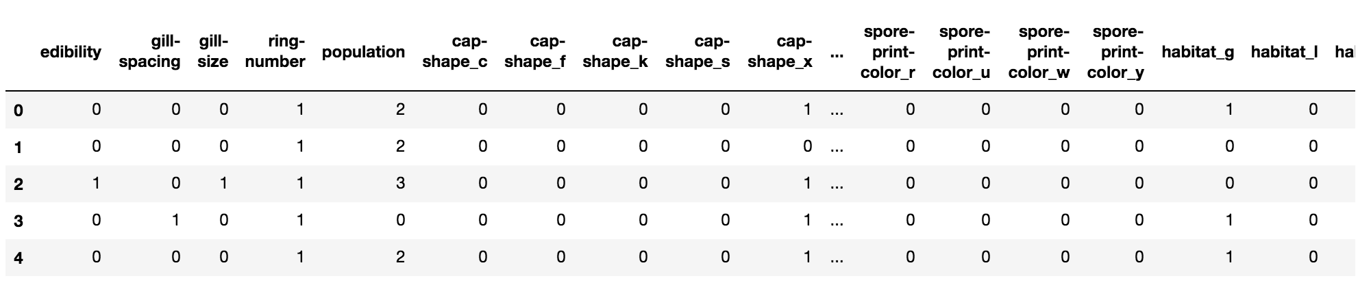
いけてますね。

データの変数化が完了したので、データをトレーニング用とテスト用に分割します。

from sklearn.model_selection import train_test_split

#トレーニングデータとテストデータに分割
(X_train, X_test, y_train, y_test) = train_test_split(mr_data_le.iloc[:,1:], mr_data_le.iloc[:,0], test_size=0.3, random_state=0)

#意図した通りにデータが分割されているか確認
print(X_train.shape,X_test.shape,y_train.shape,y_test.shape)

(5686, 90) (2437, 90) (5686,) (2437,)

いけてます。

データの準備も終わったので、モデルに学習させていきます。
今回はランダムフォレストを使用します。

from sklearn.ensemble import RandomForestRegressor

#ランダムフォレストを実行
forest = RandomForestRegressor(n_estimators=100, criterion='mse', random_state=1, n_jobs=-1)
forest.fit(X_train, y_train)
y_train_pred = forest.predict(X_train)
y_test_pred = forest.predict(X_test)

結果を表示します。

from sklearn.metrics import mean_squared_error, r2_score

#平均二乗誤差を出力
print('MSE train: %.3f, test: %.3f' % (
        mean_squared_error(y_train, y_train_pred),
        mean_squared_error(y_test, y_test_pred)))

MSE train: 0.000, test: 0.000

#決定係数を出力
print('R^2 train: %.3f, test: %.3f' % (
        r2_score(y_train, y_train_pred),
        r2_score(y_test, y_test_pred)))

R^2 train: 1.000, test: 1.000

#正解率を出力
accuracy = forest.score(X_test, y_test)
print(accuracy)

0.999940906202

ほぼ100%の精度になりました。

5.おまけの検証

あっさり精度が出てしまったのですが、おまけで気になった箇所を見ていきます。

まずは「胞子の色が毒に関連しているのでは？」という勘の検証です。

import seaborn as sns
import matplotlib.pyplot as plt

#胞子の色別で食べられるか可視化
sns.countplot(x='edibility',  hue='spore-print-color',  data=mr_data)
plt.xticks([0.0,1.0],['edible','poison']) 

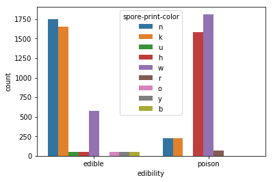
茶色と黒の多くが食べられ、一方でチョコレート色と白の多くが食べられないようです。
白は毒のイメージありますね。

続いて、匂いとの関係も見ていきます。

#匂い別で食べられるか可視化
sns.countplot(x='edibility',  hue='odor',  data=mr_data)
plt.xticks([0.0,1.0],['edible','poison']) 

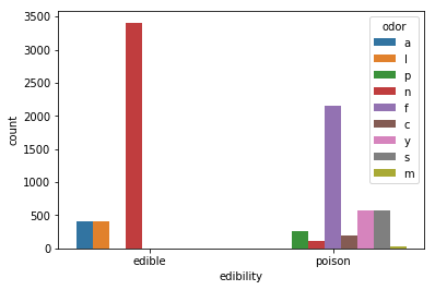
無臭のものの多くが食べられ、一方で腐った匂いのものの多くは食べられないようです。

6.おわりに

今回使用できなかった前処理のテクニックや分析手法を中心に、学んだことは今後記事として投稿しようかと思います。
最後までお読みいただきありがとうございました。
（記事にミスや改善点等ございましたらご指摘いただけると幸いです。）