Conclusion First
I exhaustively tested 144 MA crossover strategies on USDJPY 60-minute bars.
- Best full-sample result: Sharpe 0.57, cumulative return +35.45%, MaxDD -10.13%
- At first glance, it looks like a reasonably good strategy
However, when we look at the full-sample Sharpe distribution of the 144 candidates, the median is -0.277, and the 25th percentile is -1.245. In other words, most candidates have negative Sharpe ratios. A Sharpe of 0.57 is merely a number selected ex post from the right tail of the distribution.
When examined in a CSCV-like manner, the situation becomes even harsher.
- Average Sharpe of the IS-best strategy: 0.75 → 0.12 (difference -0.63; about 84% of the IS performance disappears)
- IS-OOS regression: slope = -0.556, Pearson r = -0.258, Spearman ρ = -0.339
- OOS probability of loss: 35.7% (95% Wilson confidence interval: 25.4% – 47.5%, reference value)
- Average OOS rank: 32nd / 144
- Simplified PBO: 4/70 = 5.71% (95% Wilson confidence interval: 2.2% – 13.8%, reference value)
The PBO is relatively low, but this does not mean the strategy is “safe.” PBO is a rank-based metric that checks whether the selected strategy falls into the bottom half of the candidate pool, whereas OOS probability of loss is an economic metric that checks whether the absolute return is negative. They are different concepts. If the overall quality of the candidate pool is poor, even a strategy that ranks high OOS can still have a negative absolute return.
This is exactly the point made by the framework of Bailey, Borwein, López de Prado, and Zhu (2014).
Below, I summarize the key points of the paper and the details of the experiment.
Paper URL: https://papers.ssrn.com/sol3/papers.cfm?abstract_id=2326253
1. Problem Setting: Edge Discovery Has Become “Easy” in the AI Era
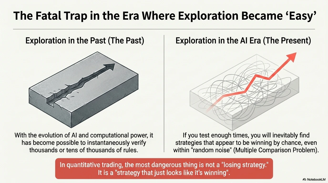
In recent years, advances in AI, Python, cloud computing, and various backtesting libraries have made edge discovery in quantitative trading far easier than before. Trading rules and features such as moving averages, RSI, Bollinger Bands, and machine learning models can now be tested in large numbers within a short period of time.
At the same time, however, the problem has become more serious: the more strategies you try, the more likely you are to find a strategy that appears to work purely by chance. This is similar to the multiple testing problem in statistics.
The authors of the paper show that by optimizing a moving average crossover strategy on a random-walk series, it is possible to create an apparently significant strategy with an annualized Sharpe ratio of 1.27. Even on a series with zero edge, if enough trials are conducted, you will inevitably find a “strategy that appears to win.”
What is truly dangerous in quantitative trading is not a losing strategy, but a strategy that only appears to be winning.
2. Backtest Overfitting and the Definition of PBO
What Is Backtest Overfitting?
Backtest overfitting is the state in which a strategy is not capturing the essential structure of the market, but is instead excessively fitted to random noise contained in past data.
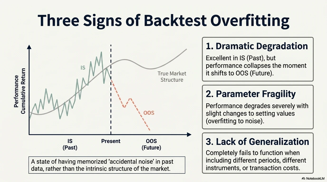
Typical symptoms are as follows:
- Excellent performance in IS, but significant deterioration in OOS
- Performance collapses when parameters are changed slightly
- The result cannot be reproduced in another period, another asset, or after costs are included
The Precise Definition of PBO

Strictly following the paper’s definition, PBO is not a measure of whether a single strategy is good or bad. Rather, it is the probability that the selection process of choosing the best strategy from N candidates fails OOS.
PBO = the probability that the strategy selected as best in IS from N candidates falls below the median of the N candidates in OOS
Therefore, a high PBO means that the best strategy obtained from that selection process is difficult to trust. The paper mentions a conventional practice of rejecting a model or selection process whose estimated PBO exceeds 0.05, but this is not a rejection of an individual strategy. Rather, it is an argument that the entire selection process should be questioned.
The important point is not to think of overfitting as a binary condition — “overfit” or “not overfit” — but to evaluate it as a probability.
3. A Counterintuitive Fact: How to Interpret IS Sharpe in a Selection Process
The paper repeatedly demonstrates an important empirical fact.
In a process that selects the candidate with the maximum IS Sharpe from many candidates, the higher the IS Sharpe, the lower the OOS Sharpe tends to be.
In Figure 2 of the paper, within the range where IS Sharpe is between 1 and 3, the regression line has a slope of -0.75 (R² = 0.17), showing a strong negative relationship. In Figure 7, which optimizes MA crossover strategies on a random walk, the slope is also negative at -0.61.
This is not a universal law that “strategies with high Sharpe ratios in the market will deteriorate in the future.” Rather, it is the phenomenon that the act of selecting the best candidate ex post from many candidates pushes up IS performance by the amount of selection bias.
In other words, a high IS Sharpe contains both:
- the strength of the genuine edge
- the strength of selection bias
And the larger the number of candidates N, the more dominant the latter becomes.
The practical implications are as follows:
- The decision “I found a strategy with Sharpe 2.0, so let’s deploy it live” may actually be a warning sign of selection bias
- The mere fact that IS Sharpe is high does not guarantee any advantage in OOS
- The more high-Sharpe results you obtain through an exploratory process, the greater the expected OOS deterioration becomes
4. PBO Alone Is Not Enough: Four Complementary Analyses
One of the paper’s important contributions is that it presents a framework for evaluating the reliability of a strategy by combining four complementary analyses, rather than looking at PBO in isolation.
| Analysis | What it looks at |
|---|---|
| (1) PBO | The probability that the IS-best strategy falls below the OOS median |
| (2) Performance degradation | The degree of deterioration in OOS Sharpe relative to IS Sharpe (regression coefficient) |
| (3) Probability of loss | The probability that the IS-best strategy incurs a loss OOS |
| (4) Stochastic dominance | Whether the IS-optimized selection is truly better than random selection |
In particular, (4) Stochastic dominance is often overlooked, but it is an extremely important perspective.
It asks the following question:
Does the OOS performance distribution of the selection process “choosing the best from N strategies” stochastically dominate the OOS performance distribution of “randomly choosing one strategy”?
If it does not, the selection process is not creating value in the first place. Figure 4 of the paper shows a case where the cumulative distribution of optimized OOS Sharpe is shifted to the left of the non-optimized distribution of OOS Sharpe across all strategies. This is strong evidence that optimization is counterproductive.
Practical checkpoints are as follows:
- Even when PBO is low, the OOS probability of loss can be high (the strategy may be bad for reasons other than overfitting)
- Even when PBO is low, if the selection process cannot dominate random selection, then the act of selection itself has no meaning
- Even if IS Sharpe is in the right tail of the distribution, if it cannot be distinguished from a random strategy in OOS, then it was not really “discovered”
5. CSCV: Holdout Alone Is Not Enough
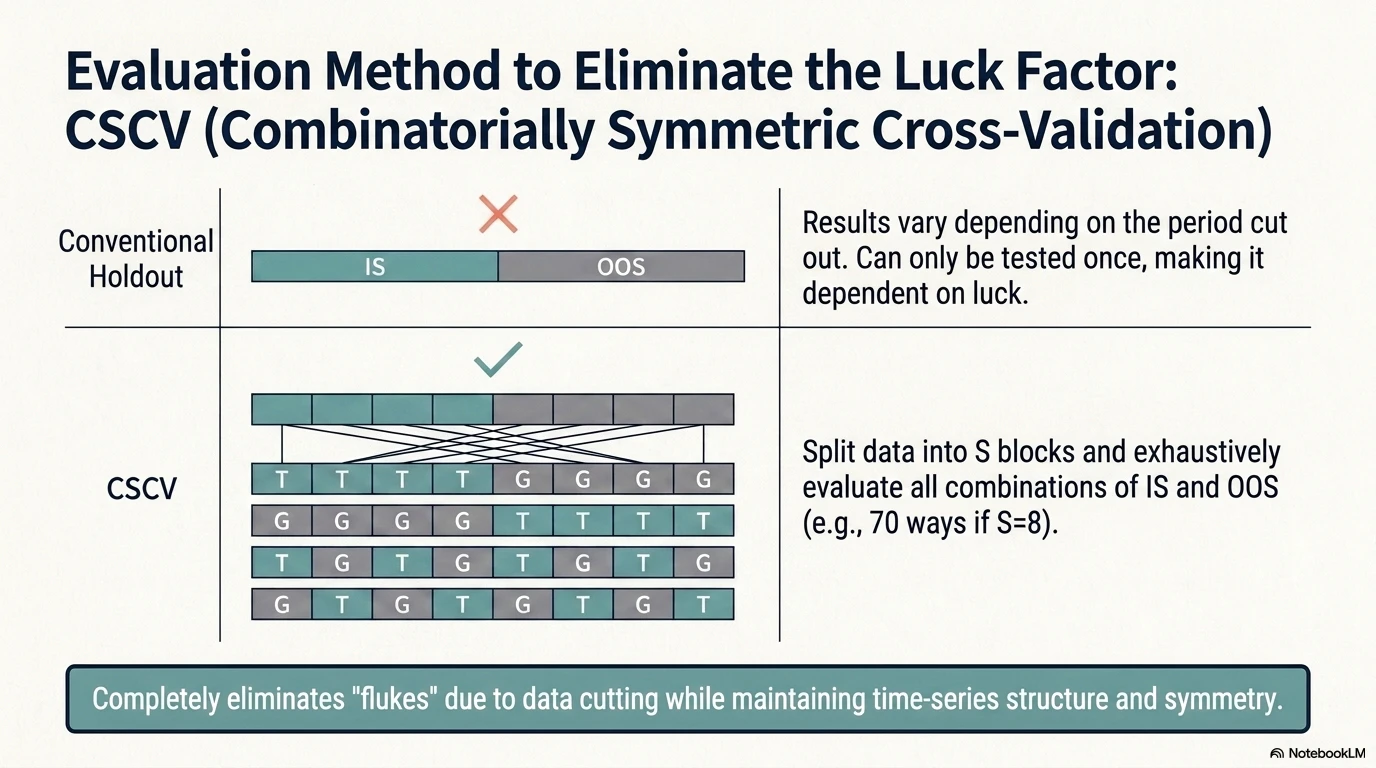
The paper proposes CSCV: Combinatorially Symmetric Cross-Validation as a method for estimating PBO.
A normal holdout has weaknesses. The result changes depending on which period is used as the holdout, evaluation becomes unstable when the sample is small, the researcher may know the characteristics of the holdout period, and the method cannot reflect overfitting caused by multiple trials.
In CSCV, the data is divided into S blocks — the paper recommends S = 16 — and S/2 blocks are used as IS while the remaining blocks are used as OOS. All combinations are evaluated. If S = 16, then ${}{16}C{8} = 12{,}870$ combinations are generated.
The advantages of CSCV are as follows:
- IS and OOS have the same size, so the estimation precision of their Sharpe ratios is aligned
- Every training set is also used as a validation set, creating symmetry
- Observations are not randomly assigned, so the time-series structure is preserved
- It is a deterministic method that always returns the same result for the same input
- The variance of the logit itself contains information about strategy robustness
If the edge is genuine, some degree of OOS advantage should remain even when the data split changes. Conversely, if the strategy is optimized to past noise, it may look strong in IS but tends to fall below the median in OOS.
6. Experiment: Simplified PBO Test on USDJPY 60-Minute Bars
Experimental Conditions
| Item | Description |
|---|---|
| Target | USDJPY 60-minute bars, based on Bid close |
| Period | 2020-01-01 to 2026-01-01 (about 6 years) |
| Data source | MT4-format 60-minute historical bars (timestamps are server time) |
| Weekend gaps | Not interpolated; preserved as natural weekend gaps (gaps_over_1h_count = 318) |
| Strategy family | Moving average crossover (long when short-term MA > long-term MA, short otherwise) |
| Short-term MA | 5, 10, 20, 30 |
| Long-term MA | 50, 100, 150, 200 |
| Stop loss | None / ATR(14) × 1.0 / × 1.5 |
| Take profit | None / ATR(14) × 1.5 / × 2.0 |
| Number of candidates | 4 × 4 × 3 × 3 = 144 strategies |
| Trading cost | Round trip 1.0 pips (0.5 pip one way); swaps and slippage not considered |
| Execution rule | Signal is judged after the close is confirmed; execution at the next bar’s open |
| Same-bar SL/TP priority | Conservatively prioritize SL |
| CSCV split | 8 blocks, IS 4 blocks / OOS 4 blocks, all ${}{8}C{4} = 70$ combinations |
The paper recommends S = 16, but given the six years of data and the priority placed on preserving the time-series structure, I use S = 8 in this experiment.
Definition of “Simplified PBO”
The PBO in this experiment differs from the paper’s formal CSCV method, which computes $\phi = \int_{-\infty}^{0} f(\lambda)d\lambda$ from the logit distribution $f(\lambda)$ based on rank-logit transformation.
For educational purposes, this experiment directly counts:
Simplified PBO = the proportion of the 70 IS/OOS splits in which the OOS rank of the IS-best strategy falls into the bottom half (ranks 73–144)
Here, rank 1 is defined as the best and rank 144 as the worst. Although this differs in detail from the formal logit-based CSCV estimate, it captures the essence of PBO: the probability that the IS-best strategy falls to the worse-than-median side in OOS. To distinguish it from the formal method, this article consistently calls it “simplified PBO.”
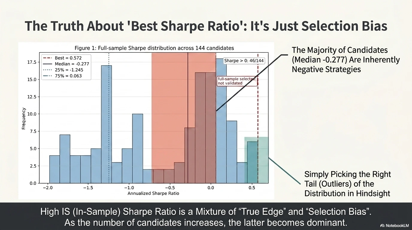
Result 1: The “Best Strategy” in the Full Sample
The figure below shows the Sharpe distribution for the 144 strategies evaluated over the full period from 2020 to 2026.
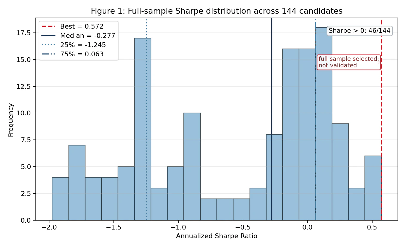
The best strategy has a Sharpe ratio of 0.572, located at the right tail of the distribution. What should be noted here is the shape of the distribution: the median of the 144 candidates is -0.277, the 25th percentile is -1.245, and even the 75th percentile is only +0.063. In other words, only 46/144 candidates (about 32%) have Sharpe > 0, meaning that two-thirds of the 144 tested strategies have negative Sharpe ratios.
Under these circumstances, selecting the “best strategy” should essentially be understood as pulling out, by chance, something located at the right tail of a distribution dominated by negative Sharpe ratios. The full-sample best strategy is located at the right tail, but it is important to note that this is “full-sample selection,” not validation (as indicated by the note in the figure: “full-sample selected; not validated”).
The top five strategies are as follows:
| Rank | Strategy | Sharpe | CumReturn | MaxDD | Trades | WinRate |
|---|---|---|---|---|---|---|
| 1 | ma_s20_l50_sl_none_tp_none | 0.5717 | 35.45% | -10.13% | 786 | 38.17% |
| 2 | ma_s20_l50_sl_atr1_5_tp_none | 0.5396 | 31.93% | -10.25% | 1659 | 30.08% |
| 3 | ma_s10_l50_sl_atr1_5_tp_none | 0.5088 | 29.41% | -11.27% | 1715 | 29.15% |
| 4 | ma_s10_l50_sl_none_tp_none | 0.4990 | 29.87% | -17.23% | 938 | 34.97% |
| 5 | ma_s10_l50_sl_atr1_0_tp_none | 0.4543 | 25.32% | -12.27% | 2271 | 24.39% |
The following chart shows the cumulative equity curve and drawdown of the best strategy. The maximum drawdown is -10.13%, with deep drawdowns occurring in the second half of 2022 and in 2025.
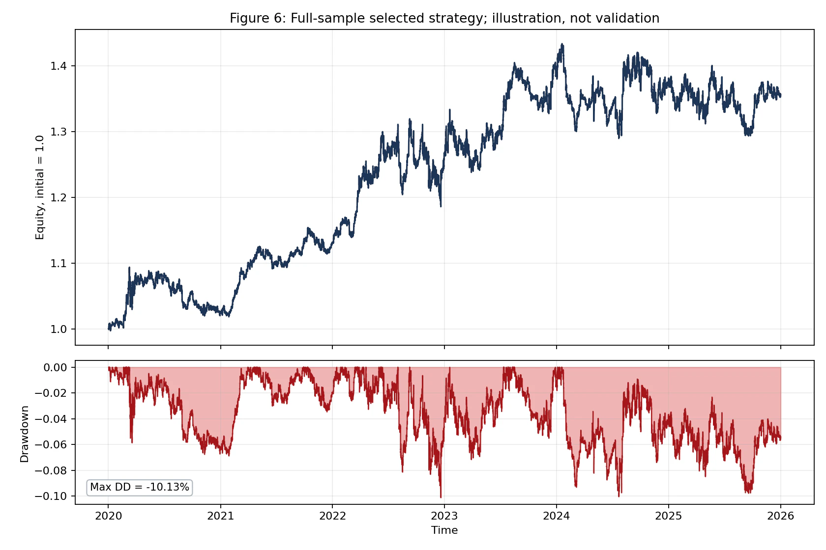
However, this is a presentation of the result after selecting the best strategy ex post, not a validation of the strategy. This is why the figure title explicitly says “illustration, not validation.” Judging that “the equity curve does not look bad” is exactly the kind of bias warned against in the paper.
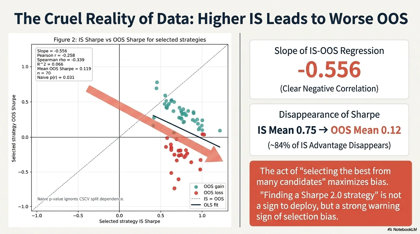
Result 2: CSCV Evaluation of the Selection Process
I evaluated all 70 IS/OOS combinations using an 8-block split. In each combination, I selected the strategy with the highest Sharpe in IS and recorded how that same strategy behaved in OOS.
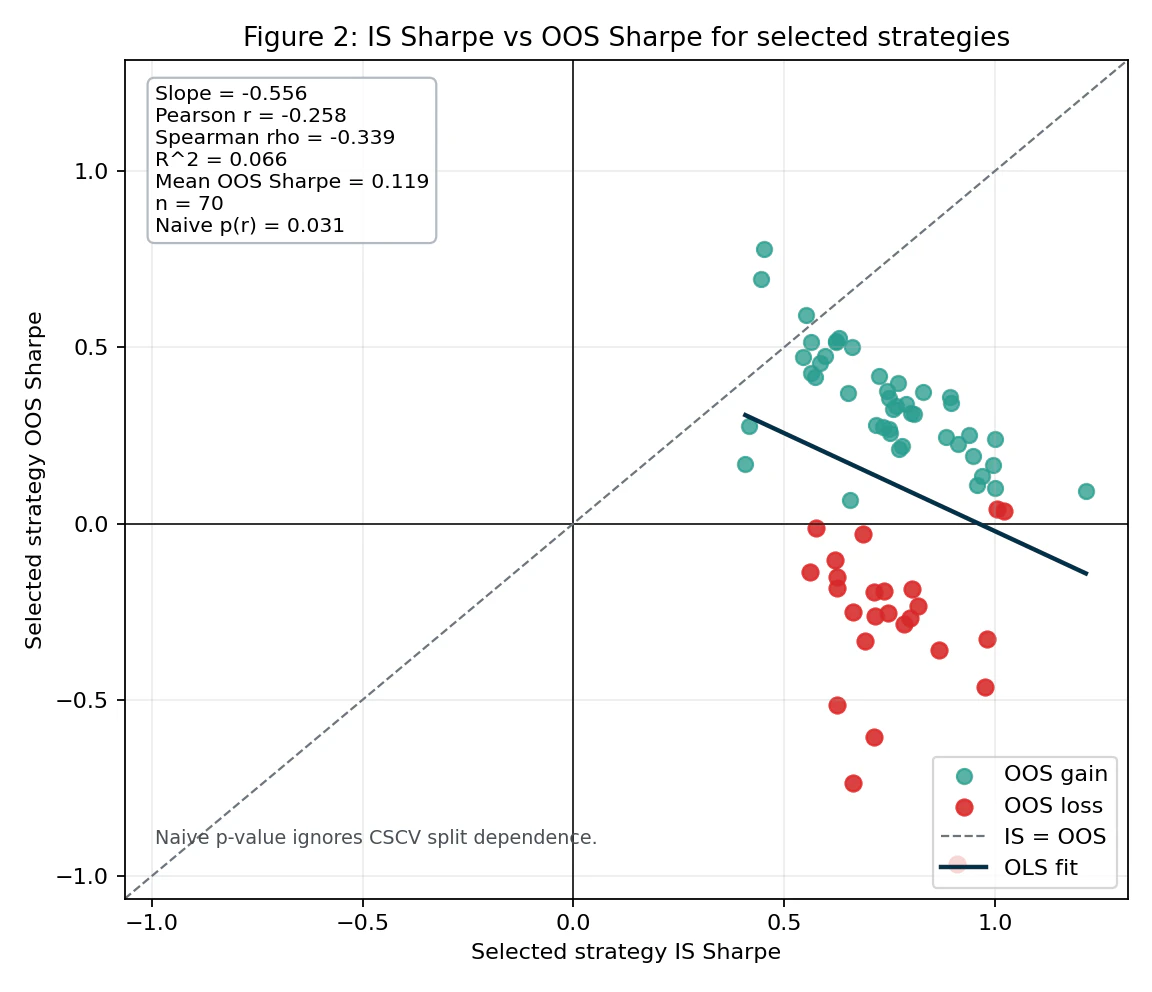
The horizontal axis is IS Sharpe, and the vertical axis is OOS Sharpe. The OLS fit shows the following statistics:
| Statistic | Value |
|---|---|
| Slope | -0.556 |
| Pearson r | -0.258 |
| Spearman ρ | -0.339 |
| R² | 0.066 |
| Mean OOS Sharpe | 0.119 |
The R² itself is small at 0.066, meaning that IS Sharpe alone cannot explain most of the variation in OOS Sharpe. However, the signs of the OLS slope, Pearson r, and Spearman ρ are all clearly negative. This confirms that:
In a process that selects the best strategy by IS Sharpe from many candidates, a high IS Sharpe does not predict a high OOS Sharpe; rather, it is weakly negatively correlated.
The figure also shows a naive p-value = 0.031 for Pearson correlation, but this should be treated only as a reference value under the assumption that the 70 trials are independent samples. CSCV splits are not mutually independent, so this p-value should not be read as a rigorous statistical test. It should be treated as an auxiliary indicator for intuitively evaluating the direction and magnitude of the correlation (see the note in the figure: “Naive p-value ignores CSCV split dependence”).
For reference, Figure 2 of the paper reports slope = -0.75 (R² = 0.17) in a similar regression, while Figure 7 (MA crossover optimization on a random walk) reports slope = -0.61 (R² = 0.04). The slope of -0.556 observed in this USDJPY 60-minute experiment is at a similar level to the negative relationships reported in the paper.
Also note that OOS gain (green) and OOS loss (red) are separated in the scatter plot. The breakdown is 45 strategies with positive OOS results and 25 strategies with negative OOS results. The height of IS Sharpe cannot distinguish between these two groups.
Numerically, the results are as follows:
| Metric | Value |
|---|---|
| Average IS Sharpe of selected strategies | 0.7474 |
| Average OOS Sharpe of selected strategies | 0.1187 |
| Average IS-OOS degradation | -0.6287 |
| Average OOS rank | 32.43 / 144 |
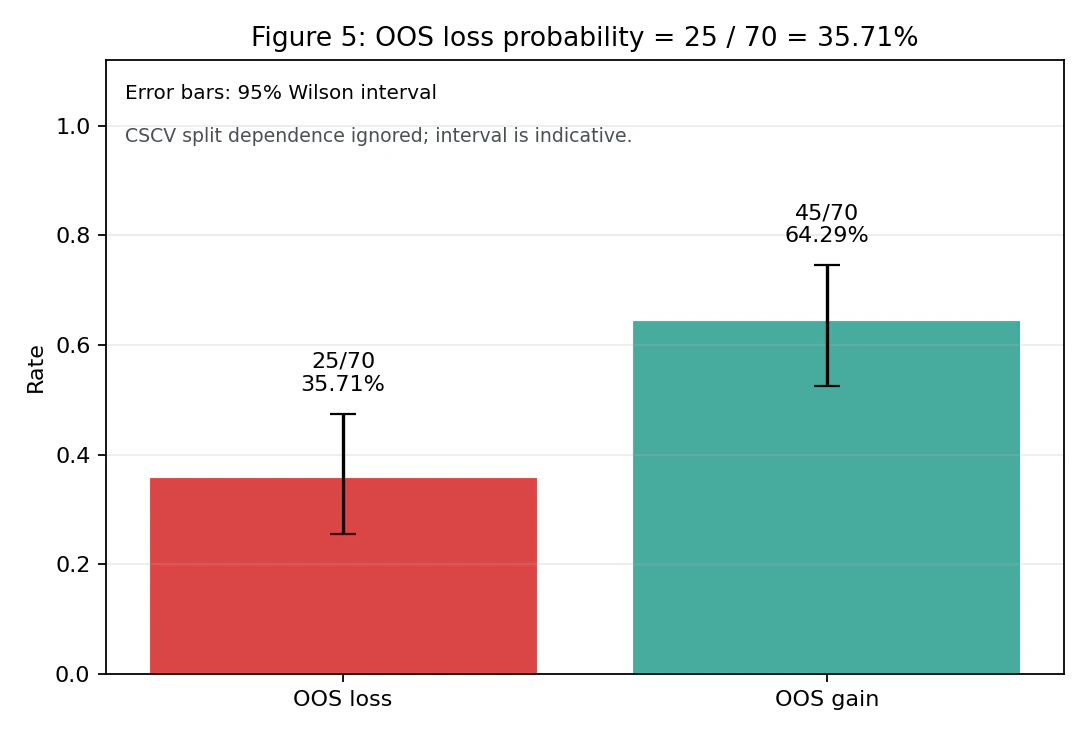
| OOS probability of loss (P[OOS CumRet < 0]) | 35.71% |
Strategies that had an average Sharpe of 0.75 in IS fell to an average of 0.12 in OOS. The degradation is about -0.63 Sharpe points, meaning that 84% of the IS performance disappeared. Furthermore, 25 of the 70 selected strategies (35.71%, 95% Wilson confidence interval: 25.4% – 47.5%, reference value) had negative cumulative OOS returns.
Result 3: Simplified PBO
The following is the OOS rank distribution of the IS-best strategies. Rank 1 is the best, and rank 144 is the worst.
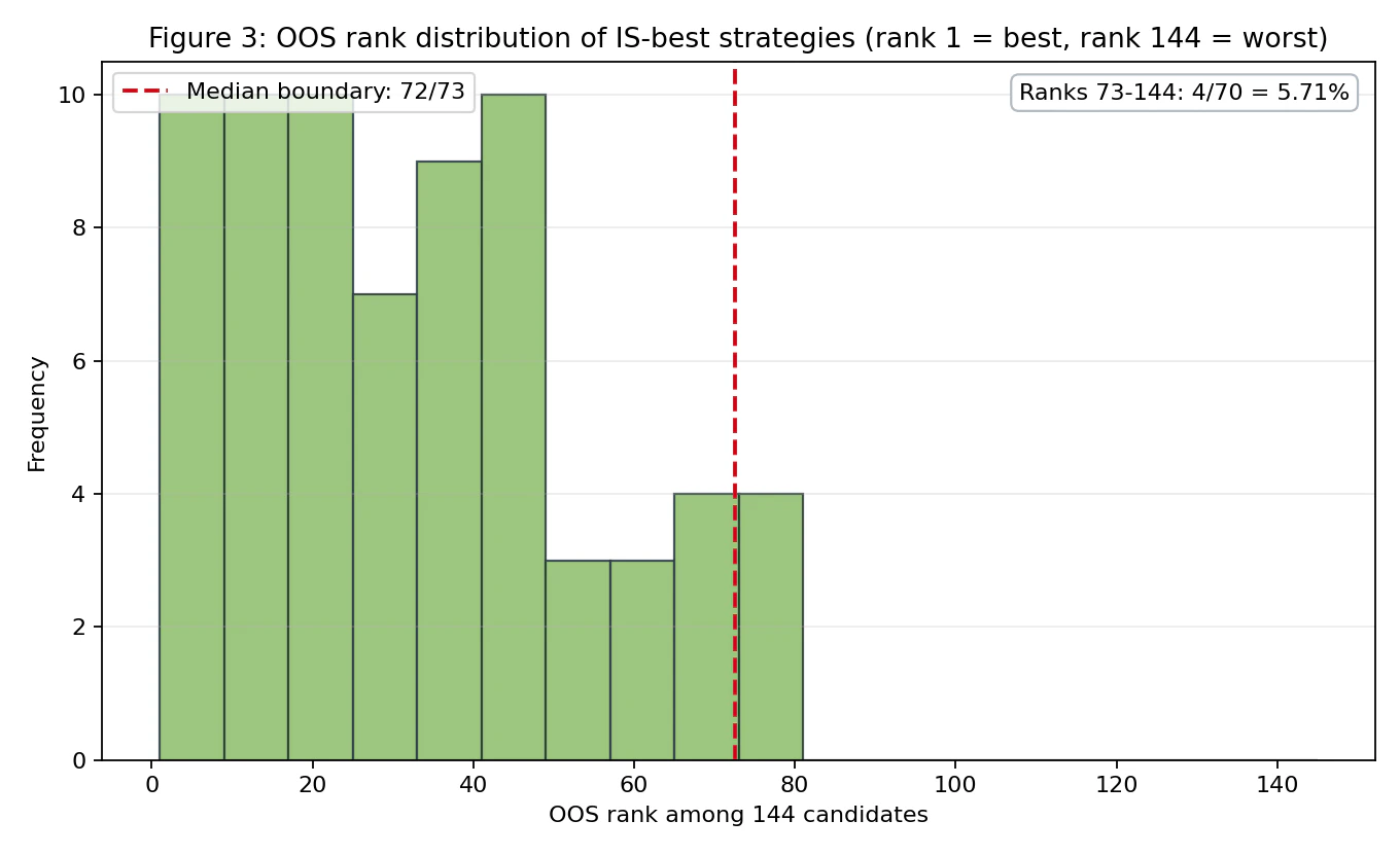
OOS ranks are mostly distributed from rank 1 to around rank 80, and there are only four cases in which the selected strategy falls into the bottom half (ranks 73–144).
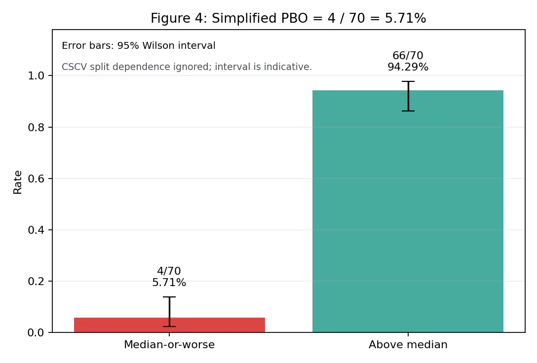
The simplified PBO is therefore 4/70 = 5.71% (95% Wilson confidence interval: 2.2% – 13.8%). The point estimate is roughly at the same level as the conventional threshold of 0.05 discussed in the paper. However, the upper bound of the Wilson confidence interval reaches 13.8%, and due to the limited sample size of 70 combinations, the uncertainty is large.
Note on Wilson intervals: The Wilson interval is a reference value that treats each split as an independent Bernoulli trial. In CSCV, the same time-series blocks are reused across multiple combinations, so there is strong dependence among the splits. Therefore, this interval is not a rigorous confidence interval; it should be read as an auxiliary indicator that intuitively shows the uncertainty of the point estimate. The same applies to the OOS loss probability of 35.7%.
If the paper’s recommended S = 16 were used, the number of combinations would increase to ${}{16}C{8} = 12{,}870$, and the logit and rank distributions could be estimated more smoothly. However, even if the number of combinations increases, the splits are not independent. Therefore, it should not be interpreted simply as “the effective sample size becomes 12,870.” The S = 8 / 70-combination design in this experiment was chosen as a trade-off with preserving the time-series structure, but it is not sufficient from the perspective of PBO estimation precision.
Result 4: How to Read the Four-Metric Set
Following the paper’s framework, the four metrics can be arranged as follows:
| Analysis | Result in this experiment | Interpretation |
|---|---|---|
| (1) Simplified PBO | 5.71% (95% CI: 2.2% – 13.8%) | Falling below the median is rare, but the CI is wide |
| (2) Performance degradation | IS 0.75 → OOS 0.12 (slope -0.556, R² 0.066) | The negative slope is clear, and the degradation is large |
| (3) Probability of loss | 35.71% (95% CI: 25.4% – 47.5%) | More than one in three cases end with negative cumulative return |
| (4) Stochastic dominance | Not implemented (for next time) | Not examined in this experiment |
Stochastic dominance in (4) is the analysis that checks whether the OOS distribution of the selected strategy dominates the OOS distribution obtained by randomly selecting one strategy. This was not implemented in the present experiment, but it is an essential metric for completing the framework of the paper. I leave it as a task for next time.
Rank-Based Metrics and Economic Metrics Are Different
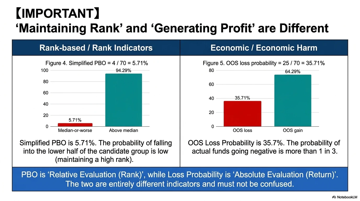
The most important point in this experiment is that despite a low PBO, the OOS probability of loss is 35.71%. This is not a contradiction.
- PBO is a rank-based metric that asks whether the selected strategy falls into the bottom half of the candidate pool
- OOS probability of loss is an economic metric that asks whether the absolute return becomes negative
They are different concepts. If the overall quality of the candidate pool is low, even a high OOS rank may correspond to low or even negative absolute returns.
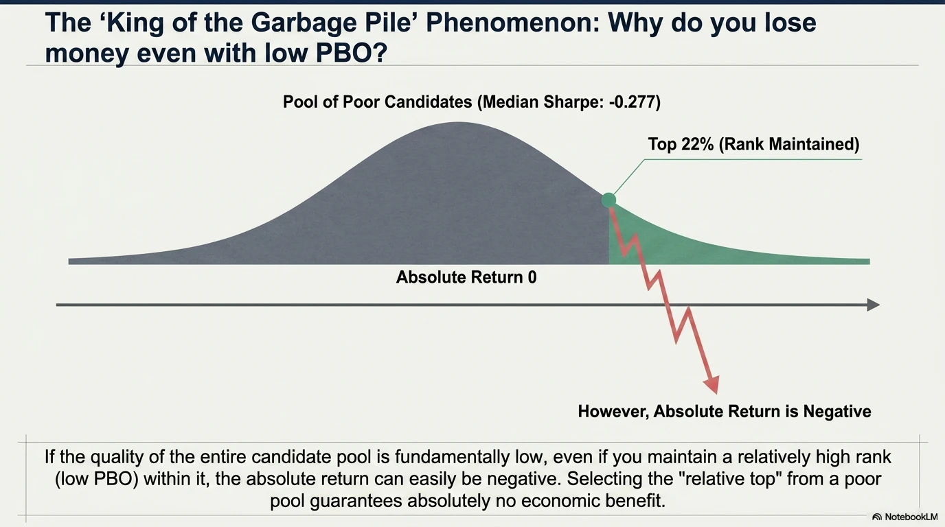
This experiment is exactly such a situation. The median full-sample Sharpe of the 144 candidates is -0.277, meaning that the candidate pool itself is poor. Even if we select a strategy that is “relatively high-ranking” from this poor pool, there is no guarantee that its absolute return will be stably positive. “High OOS rank (rank 32) = safe” is not true; “high rank but negative in absolute terms” occurs frequently.
This is an important fact that is missed when looking only at PBO.
How to Read the Numbers
It is important not to misunderstand the results.
We cannot say, “PBO is 5.7%, so it is not overfitted.”
The observed facts can be summarized as follows:
- The candidate pool itself is poor: the median Sharpe of the 144 strategies is -0.277, and the 25th percentile is -1.245. We are selecting the right tail ex post from a distribution where negative Sharpe ratios are the majority
- PBO is low (point estimate 5.71%, Wilson CI upper bound 13.8%, reference value): the probability that the selection process causes the IS-best strategy to fall into the bottom half OOS (ranks 73–144) is small
- IS-OOS is weakly negatively correlated (slope -0.556, Spearman -0.339, R² 0.066): high IS Sharpe does not predict high OOS Sharpe
- OOS Sharpe deteriorates to an average of 0.12: 84% of the advantage seen in IS disappears
- OOS probability of loss is 35.71% (reference CI 25.4%–47.5%): the selected strategy loses money in future periods more than one-third of the time
- Average OOS rank is 32nd: even if we select the “best strategy in IS,” it lands around the top 22% in OOS
- High rank ≠ economic advantage: because the candidate pool is poor, even a high OOS rank can have a negative absolute return
In other words, this MA crossover strategy family is not as severely flawed as a case of “complete overfitting,” but it is clear that the IS Sharpe should not be expected to persist into the future as-is.
If one were to deploy a strategy live with small capital after observing an IS Sharpe of 0.75, the honest expectation would be something like a Sharpe around 0.1 in reality, with more than a 30% probability of negative cumulative return.
This phenomenon is observed even with a relatively modest exploration of 144 candidates. If AI is used to generate thousands or tens of thousands of rules, PBO and the other metrics may deteriorate further.
However, what matters here is not the number of candidates N itself, but the effective number of trials, taking into account the correlations among candidates. Even if AI generates 10,000 rules, if they are all variants of similar MA crossovers, the number of independent trials is not 10,000. Conversely, if the feature space, target assets, timeframes, and model structures expand, the effective number of trials grows, and selection bias becomes more serious.
A claim such as “We tried N = 10,000 rules and got Sharpe 2.0” can fall into two extremes:
- If the rules are variants of almost the same logic, it is effectively equivalent to only several dozen trials
- If the rules span diverse features, markets, and timeframes and are close to independent trials, then it may really be close to N = 10,000
When evaluating PBO or MinBTL, it is therefore necessary to also examine the diversity of the candidate pool.
Also, this experiment is not AI-driven exploration, but a manually defined grid search. The 144 MA crossover candidates are combinations of short-term MA × long-term MA × SL × TP, so they are a highly correlated family of variants. The effective number of trials is clearly smaller than 144. How PBO behaves for AI-generated rules, and how to measure the effective number of trials, are important topics that should be compared, but this article does not address them. This is also a task for next time.
7. What Should Still Not Be Trusted in This Experiment
The experiment in this article is an educational validation for understanding the behavior of PBO, and it is not a trading recommendation for any specific MA crossover strategy. For professional quant readers, I explicitly disclose the elements not incorporated in this experiment.
Data and Execution Factors Not Considered
- Data vendor differences: USDJPY 60-minute bars differ by vendor in whether they are based on Bid, Ask, or Mid prices, as well as rounding and missing-data handling. Running the same strategy on data from another vendor can change the result
- Spread variation: This experiment uses a fixed round-trip cost of 1.0 pips. In reality, spreads vary substantially by time of day, market conditions, and volatility, and can widen severalfold during early Tokyo hours, the London close, or news events
- Execution slippage: The experiment assumes execution at the next bar’s open, but actual market orders experience slippage. Trend-following strategies such as MA crossovers are particularly prone to unfavorable slippage
- Swaps and interest-rate differentials: USDJPY carry can have a large effect on results. For long-holding strategies, swaps can become a major source of returns, and this experiment completely ignores them
- Holiday and weekend handling: Weekend gaps were left as natural gaps without interpolation, but depending on the vendor or execution environment, Monday-opening gap executions may occur
- Bar construction time: Whether 60-minute bars are cut by UTC or by server time changes the timing of signals
- ATR definition: This experiment uses ATR(14), but the value differs depending on whether Wilder smoothing or a simple moving average is used. The sensitivity of SL/TP levels depends on this
- Position size and leverage: This experiment uses a simple unit-trade assumption. In actual trading, results change greatly with risk parity or Kelly-style sizing
- Taxes: For Japanese residents, the taxation method differs between OTC FX and Click 365, and after-tax returns are effectively smaller
These are not “negligible errors.” They are factors that can move the Sharpe estimate itself. The full-sample Sharpe of 0.57 observed here could easily shrink toward zero if these factors were included.
Limitations of the Validation Method
- Small number of combinations: S = 8 / 70 combinations: The paper recommends S = 16 / 12,870 combinations. The 95% Wilson CI for the PBO estimate in this experiment is wide at 2.2% – 13.8%, so it cannot distinguish between 5% and 14%
- Not formal CSCV: The formal method in the paper computes $\phi = \int_{-\infty}^{0} f(\lambda)d\lambda$ from the logit distribution $f(\lambda)$. This experiment uses a simplified direct count of the proportion of cases in which the OOS rank of the IS-best strategy falls into the bottom half (ranks 73–144), and may differ in detail from the paper’s estimate
- Stochastic dominance not implemented: Of the four-metric framework in the paper, this experiment does not test whether the selection process stochastically dominates random selection
- Single asset and single timeframe: Only USDJPY 60-minute bars are used. Reproducibility on EURUSD, daily bars, 5-minute bars, and so on has not been tested
- Structural regime changes not considered: The 2020–2026 period includes regime shifts such as the COVID shock, the transition from low to high interest rates, and the depreciation of the yen. CSCV across these regimes can also be interpreted as “mixing different market environments,” so the meaning of the result should be treated carefully
- CSCV does not imitate the time-series production process: Depending on the combination, later blocks in the time series can enter IS while earlier blocks enter OOS. Therefore, CSCV is not a “backtest that predicts the future”; it is a post hoc diagnostic for how fragile the process of selecting the best strategy from many candidates is to the way the data is split. Before live deployment, separate Walk-Forward Optimization and a completely untouched holdout are necessary
Reproducibility
The experimental code (run_backtest_overfitting_experiment.py) is written to run deterministically with NumPy, and the same CSV input should produce the same results. No random numbers are used (MA crossover, ATR, and cost calculations are all deterministic). However, the final decimal places may vary due to the enumeration order of CSCV combinations, Python version, rounding errors, and similar factors.
In short, the numbers in this article are reference values for observing how the paper’s PBO framework behaves on real USDJPY data, not validations robust enough for live trading. Actual trading decisions require additional validation incorporating all of the factors above.
8. An Important Prohibition: Do Not Use PBO as an Objective Function
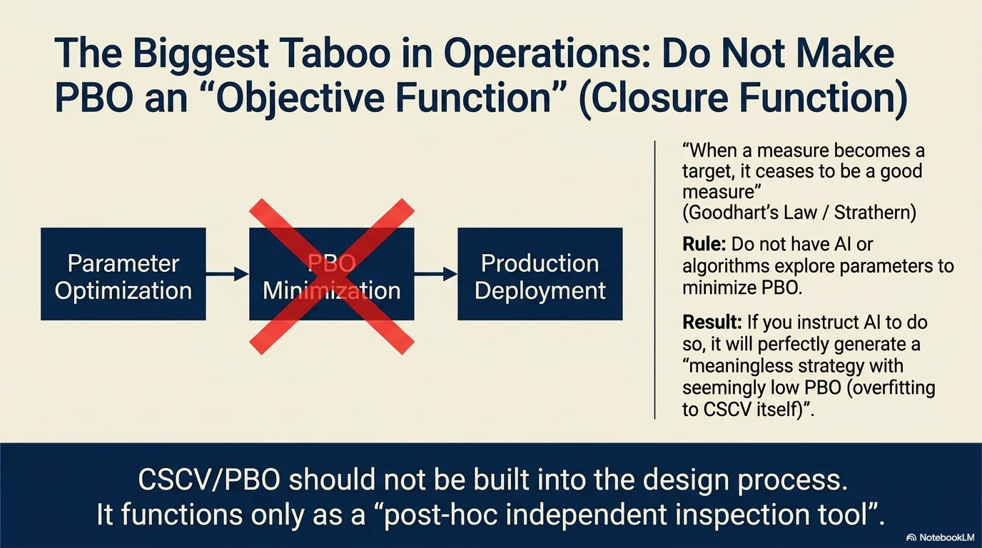
In Section 5.2 of the paper, the authors issue a strong warning.
“When a measure becomes a target, it ceases to be a good measure.” (Strathern, 1997)
Once a metric becomes a target, it is no longer a good metric.
Specifically, the following uses are prohibited:
- ❌ Selecting a strategy with an optimization algorithm that minimizes PBO
- ❌ Incorporating CSCV as an objective function for parameter tuning
- ❌ Filtering multiple strategy candidates by PBO and then re-optimizing the remaining strategies
This is because the moment CSCV becomes the optimization target, overfitting to CSCV itself begins. Even if parameters that minimize PBO are found, that only means they are overfitted to the “PBO test,” not that they represent a genuine edge.
CSCV is a tool for post hoc evaluation of the quality of a strategy-selection process, and it must not be incorporated inside the process of selecting a strategy.
This trap is especially serious in the AI era. If you instruct AI to “find the strategy parameters that minimize PBO,” the AI will happily search for them. But the output will merely have a superficially low PBO and will not work in production.
The rule is simple:
CSCV is inspection, not design.
9. PBO’s Siblings: MinBTL and the Deflated Sharpe Ratio
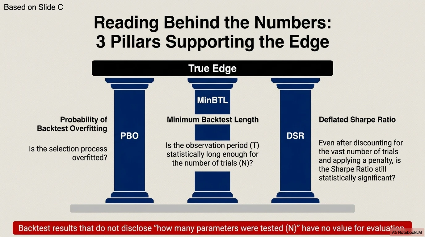
As metrics that should be reported together with PBO, the conclusion of the paper mentions MinBTL (Minimum Backtest Length) and DSR (Deflated Sharpe Ratio).
The intuition is as follows:
- If N strategies are tested, the best Sharpe among them must exceed the level that “could arise from random noise alone”
- The larger the number of trials N, the longer the observation period needed for the Sharpe ratio to be statistically significant
- Results from large-scale searches over short periods are almost certainly noise
In practice, when looking at a backtest result, the following three points must be checked together:
- PBO: whether the selection process is overfitted
- MinBTL: whether the observation period is sufficiently long relative to the number of trials N
- DSR: whether the Sharpe ratio adjusted for the number of trials is significant
For details, see López de Prado’s related paper, “The Deflated Sharpe Ratio” (2014).
The lesson here is simple:
You cannot judge from the number “Sharpe 2.0” alone.
Only after knowing “Sharpe 2.0 after how many trials?” and “over how many years of data?” can the discussion begin.
10. Implications for Quant Traders in the AI Era
Using AI can make the following tasks more efficient:
- Generating candidate trading rules and exploring features
- Testing combinations of technical indicators and optimizing parameters
- Automating backtests and summarizing and visualizing results
This is extremely powerful. However, the more AI increases the number of searches, the greater the risk of backtest overfitting becomes.
In quant development in the AI era, the following process becomes important:
- Generate edge candidates with AI
- Conduct primary validation by backtesting
- Include trading costs, spreads, and slippage
- Check stability around parameter neighborhoods
- Validate using Walk-Forward Optimization (WFO)
- Do not touch the holdout period until the end
- Examine overfitting risk using CSCV-style thinking (do not make it an objective function)
- Evaluate all four metrics together: PBO, performance degradation, loss probability, and stochastic dominance
- Be aware of the relationship between the number of trials N and the observation period T (MinBTL)
- Confirm performance in real time through DryRun
- Deploy live with small capital
- Stop and re-evaluate when performance deteriorates
11. Practical Checkpoints
When examining backtest results, at minimum, the following points must be checked:
- How many strategies and parameter combinations were tested (disclosure of the number of trials N is essential)
- Whether failed validation results are also recorded (to address the file drawer problem)
- How much performance deteriorated from IS to OOS (whether a negative slope appears)
- How high the probability of loss is in OOS
- Whether the optimized strategy is truly superior to a randomly selected strategy (stochastic dominance)
- Whether performance remains when parameters are changed slightly
- Whether performance remains when the period, currency pair, or asset is changed
- Whether performance remains after spreads and slippage are included
- Whether there is no data leakage (use of future information, or a time-series mismatch between entry signal and execution price)
Quant beginners in particular tend to be fascinated by “the backtest that performed the best.” In practice, however, what matters more than the best result is why that result appeared, under what conditions it breaks, and how reproducible it is.
12. The Core Message for Investors
What matters for investors is not a flashy backtest result. What truly matters is how well the strategy can withstand future uncertainty.
The more perfectly a strategy fits past data, the weaker it may be in the future. Conversely, even if a strategy’s past performance is only moderate, a strategy that remains stable across multiple periods, multiple conditions, and multiple validation methods may be more trustworthy in practice.
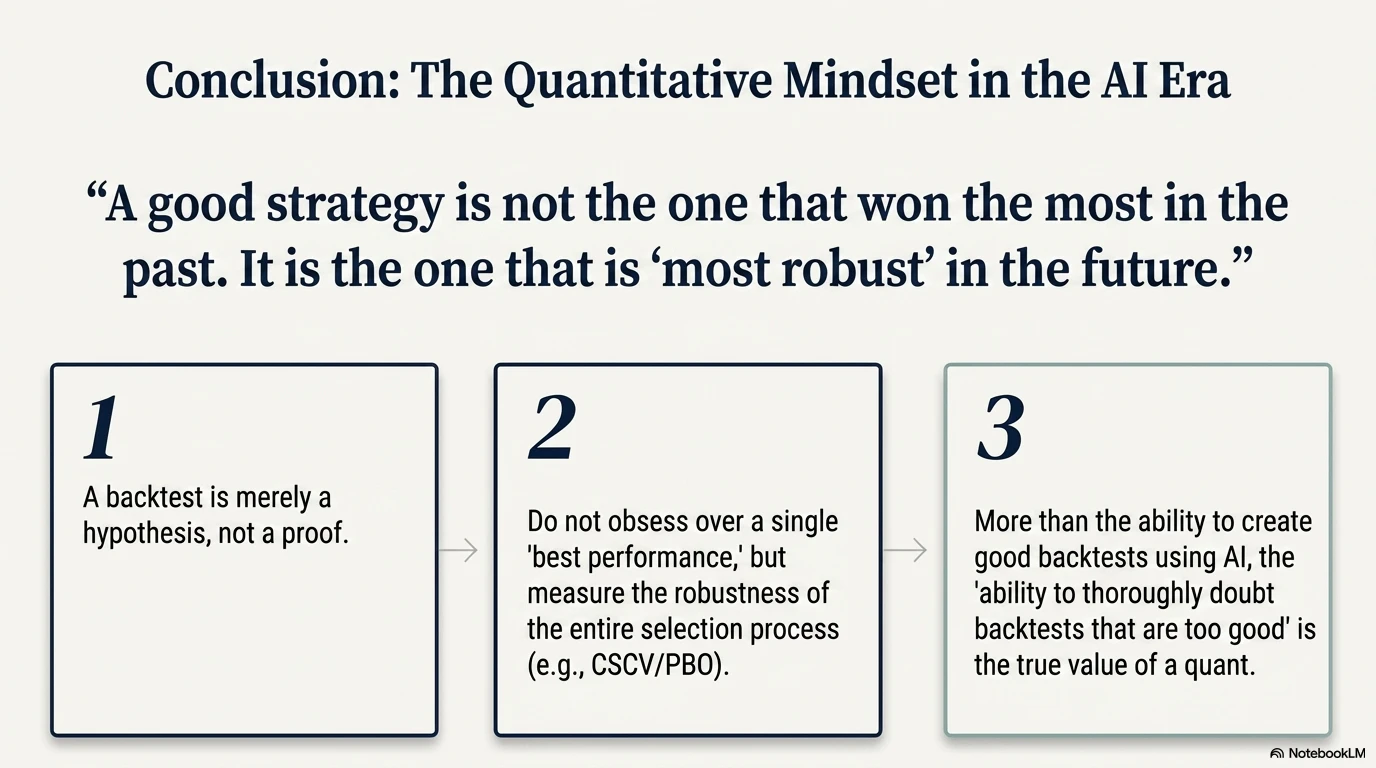
A good strategy is not the strategy that won the most in the past, but the strategy that is least likely to break in the future.
In the AI era, it will become easy to create backtests that look good. That is why both investors and developers must look not only at the backtest performance itself, but also at the validation process through which that performance was obtained.
13. Summary
The key points of this article are as follows:
- In a process that selects the best candidate ex post from many candidates, high IS Sharpe may reflect the strength of selection bias (a negative regression relationship)
- Overfitting should not be treated as a binary condition, but evaluated as a probability (PBO). PBO is not a metric for an individual strategy, but for the selection process
- PBO is a rank-based metric, while OOS probability of loss is an economic metric, and the two are different. Even with low PBO, if the overall quality of the candidate pool is poor, the probability of loss can be high
- PBO is one of four complementary analyses, and must be considered together with performance degradation, loss probability, and stochastic dominance
- CSCV is a post hoc inspection tool, and must not be used as an optimization objective function
- Numbers have no meaning unless the number of trials N, observation period T, and MinBTL are discussed together. Ideally, the analysis should also go further and consider the effective number of trials, accounting for correlations among candidates
Even in this simplified experiment, with a modest search of 144 candidates, a deterioration from IS Sharpe 0.75 to OOS Sharpe 0.12 was observed (difference -0.63, slope -0.556). PBO itself is relatively low at 5.71% (CI upper bound 13.8%, reference value), but the OOS probability of loss is 35.71%. “Low PBO = safe” is not true; multiple metrics must be interpreted together.
A good strategy is not the strategy that won the most in the past, but the strategy that is least likely to break in the future.
Backtesting is necessary. But backtesting is not proof.
In quant trading in the AI era, what matters is not only the ability to create a good backtest. Rather, what matters even more is the ability to doubt a backtest that looks too good.
Tasks for Next Time
Here are the topics that could not be covered in this article:
- Implementation of stochastic dominance: Check using ECDF and SD1/SD2 whether the OOS distribution of the selected strategy dominates the OOS distribution of random selection
- Implementation of formal CSCV (logit distribution): Compute $\phi = \int_{-\infty}^{0} f(\lambda)d\lambda$ using S = 16 and 12,870 combinations
- PBO comparison for AI-generated rules: Empirically examine how PBO and the four metrics change for manual grid search versus AI-generated features
- PBO sensitivity to the number of trials N: Conduct a scaling experiment on how PBO deteriorates for N = 10, 100, 1000, and 10000
- Self-implementation of MinBTL and DSR: Re-evaluate Sharpe significance on this USDJPY dataset while accounting for the number of trials N
- Estimation of the effective number of trials (effective N): Estimate how many effective trials the 144 candidates in this experiment correspond to after accounting for correlations. One possible method is to estimate effective N from the eigenvalue decomposition of the return correlation matrix among candidates
References
- Bailey, D. H., Borwein, J. M., López de Prado, M., & Zhu, Q. J. (2014). The Probability of Backtest Overfitting. SSRN. https://papers.ssrn.com/sol3/papers.cfm?abstract_id=2326253
- Bailey, D. H., & López de Prado, M. (2014). The Deflated Sharpe Ratio: Correcting for Selection Bias, Backtest Overfitting and Non-Normality. Journal of Portfolio Management, 40(5), 94-107.
- López de Prado, M. (2018). Advances in Financial Machine Learning. Wiley.
Appendix: Experimental Code and Data
Please download and use the Python code, datasets, and detailed graphs used in this experiment from the GitHub repository below.
Experiment: Lab_4
https://github.com/tikeda123/article_lab
The code, CSV files, and figures used in this article are organized as follows:
-
run_backtest_overfitting_experiment.py: Reproducibility code -
candidate_summary.csv: Full-sample evaluation of the 144 strategy candidates -
pbo_results.csv: Results of the 70 IS/OOS validations -
experiment_summary.xlsx: Integrated summary of results
Experimental Figures (Real Data)
-
fig1_sharpe_distribution.png: Full-sample Sharpe distribution -
fig2_is_vs_oos_sharpe.png: IS vs OOS Sharpe scatter plot of selected strategies -
fig3_oos_rank_distribution.png: OOS rank distribution -
fig4_simplified_pbo.png: Simplified PBO -
fig5_oos_loss_probability.png: OOS probability of loss -
fig6_best_strategy_equity_curve.png: Equity curve of the best strategy
Conceptual Figures (Generated with NotebookLM)
-
bjp1.pngtobjp14.png: Conceptual explanatory figures used in this article
Sharpe Ratio Calculation Specification
Since the impression of the Sharpe ratio for USDJPY 60-minute bars changes depending on the annualization factor, I explicitly state the calculation specification used in this experiment.
| Item | Specification |
|---|---|
| Return definition | simple return (price change rate) |
| Calculation unit | Return per bar (60 minutes) |
| Annualization factor | $\sqrt{6048}$ (explained below) |
| Sharpe formula | $SR = \mu / \sigma \times \sqrt{6048}$ (risk-free rate = 0) |
| Position state | Single position only. Reverse on opposite signal; after SL/TP is triggered, re-entry is possible from the next bar onward |
| No-position periods | Included in the series as return = 0 (reflecting the sparsity of trading opportunities) |
| Trading cost deduction | Deduct the P&L equivalent of round-trip 1.0 pip (= 0.01 yen) at execution |
| SL/TP judgment | Judged using the bar’s High/Low. If both are touched in the same bar, SL is prioritized |
| Short execution | Bid data only is used. Ask-Bid spread is incorporated into trading cost |
Basis for the annualization factor $\sqrt{6048}$: USDJPY is traded 24 hours on weekdays, with approximately 252 business days per year and 24 bars per day, giving 6,048 bars per year. Since weekends and holidays are excluded, the conversion is based on the actual number of bars rather than calendar time.
This conversion is approximate and does not strictly reflect actual tradable hours, such as the Tokyo, London, and New York market overlaps. Depending on the vendor and market-hours definition, a difference of roughly ±10% in the conversion factor may occur.