Pythonで統計のお勉強：いろんな分布を眺めてみる

準備

import numpy as np
import scipy
import matplotlib.pyplot as plt
%matplotlib inline
import seaborn as sns
sns.set(font='Kozuka Gothic Pro', style="whitegrid")

def print_ex(str, num):
    print(f"{str}は {num} です。")

def describe_list(list):
    print_ex("　　　和", np.sum(list))
    print_ex("　　平均", np.mean(list))
    print_ex("　　分散", np.var(list))
    print_ex("標準偏差", np.std(list))
    print_ex("　　歪度", scipy.stats.skew(list))
    print_ex("　　尖度", scipy.stats.kurtosis(list))
    print_ex("　最大値", np.max(list))
    print_ex("　中央値", np.median(list))
    print_ex("　最小値", np.min(list))

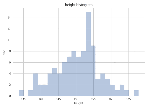
ヒストグラム

height = np.array([
    148.7, 149.5, 133.7, 157.9, 154.2, 147.8, 154.6, 159.1, 148.2, 153.1,
    138.2, 138.7, 143.5, 153.2, 150.2, 157.3, 145.1, 157.2, 152.3, 148.3,
    152.0, 146.0, 151.5, 139.4, 158.8, 147.6, 144.0, 145.8, 155.4, 155.5,
    153.6, 138.5, 147.1, 149.6, 160.9, 148.9, 157.5, 155.1, 138.9, 153.0,
    153.9, 150.9, 144.4, 160.3, 153.4, 163.0, 150.9, 153.3, 146.6, 153.3,
    152.3, 153.3, 142.8, 149.0, 149.4, 156.5, 141.7, 146.2, 151.0, 156.5,
    150.8, 141.0, 149.0, 163.2, 144.1, 147.1, 167.9, 155.3, 142.9, 148.7,
    164.8, 154.1, 150.4, 154.2, 161.4, 155.0, 146.8, 154.2, 152.7, 149.7,
    151.5, 154.5, 156.8, 150.3, 143.2, 149.5, 145.6, 140.4, 136.5, 146.9,
    158.9, 144.4, 148.1, 155.5, 152.4, 153.3, 142.3, 155.3, 153.1, 152.3
])

describe_list(height)

fig = plt.figure()
ax = fig.add_subplot(1,1,1)
ax.set_title('height histogram')
ax.set_ylabel('freq')
sns.distplot(height, kde=False, rug=False, bins=25, axlabel="height")
None

　　　和は 15062.699999999999 です。
　　平均は 150.62699999999998 です。
　　分散は 41.389571000000025 です。
標準偏差は 6.433472701426503 です。
　　歪度は -0.11463683645167477 です。
　　尖度は 0.03758292177634992 です。
　最大値は 167.9 です。
　中央値は 150.95 です。
　最小値は 133.7 です。

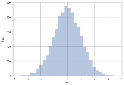
一様分布

rand = np.random.rand(10000) * 256

fig = plt.figure()
ax = fig.add_subplot(1,1,1)
ax.set_xlabel('rand')
ax.set_ylabel('freq')
sns.distplot(rand, kde=False, rug=False, bins=32)
describe_list(rand)
None

　　　和は 1274007.8689326535 です。
　　平均は 127.40078689326535 です。
　　分散は 5463.047050875183 です。
標準偏差は 73.91242825719625 です。
　　歪度は 0.01778191661125858 です。
　　尖度は -1.199422974882133 です。
　最大値は 255.9926260024685 です。
　中央値は 126.60092345500796 です。
　最小値は 0.03771370033149424 です。

正規分布

randn = np.random.randn(10000)

fig = plt.figure()
ax = fig.add_subplot(1,1,1)
ax.set_xlabel('rand')
ax.set_ylabel('freq')
sns.distplot(randn, kde=False, rug=False, bins=32)
describe_list(randn) # 平均は0、標準偏差は1になるはず
None

　　　和は -55.05329222007835 です。
　　平均は -0.005505329222007835 です。
　　分散は 0.9872874021026111 です。
標準偏差は 0.993623370348449 です。
　　歪度は -0.02209390746763633 です。
　　尖度は -0.01793660437045741 です。
　最大値は 3.692976210882958 です。
　中央値は -0.008153753688576954 です。
　最小値は -3.6868597391773084 です。

rand_normal = np.random.normal(100, 20, 10000)

fig = plt.figure()
ax = fig.add_subplot(1,1,1)
ax.set_xlabel('rand')
ax.set_ylabel('freq')
sns.distplot(rand_normal, kde=False, rug=False, bins=32)
describe_list(rand_normal) # 平均は100、標準偏差は20になるはず
None

　　　和は 1001723.9448072708 です。
　　平均は 100.17239448072708 です。
　　分散は 399.13414120433924 です。
標準偏差は 19.978341803171233 です。
　　歪度は 0.005551138939298525 です。
　　尖度は 0.11141597033179007 です。
　最大値は 183.34911533462218 です。
　中央値は 99.83668416351375 です。
　最小値は 15.019704621470993 です。

二項分布

coin_test = np.random.binomial(n=1, p=0.5, size=20)
print(coin_test)

# サイコロを1000回振ると6はどのぐらい出るのか
dice = np.random.binomial(n=1000, p=1/6, size=10000)

fig = plt.figure()
ax = fig.add_subplot(1,1,1)
ax.set_xlabel('回数')
ax.set_ylabel('freq')
sns.distplot(dice, kde=False, rug=False, bins=32)
describe_list(dice)
None

[1 1 0 1 1 1 0 1 1 1 1 0 1 0 1 1 1 0 1 1]
　　　和は 1667333 です。
　　平均は 166.7333 です。
　　分散は 138.04857110999998 です。
標準偏差は 11.749407266326246 です。
　　歪度は 0.03404297794364515 です。
　　尖度は -0.05696433202624451 です。
　最大値は 217 です。
　中央値は 167.0 です。
　最小値は 120 です。

パレート分布

pareto = np.random.pareto(a=2.718281828, size=10000)

fig = plt.figure()
ax = fig.add_subplot(1,1,1)
ax.set_ylabel('freq')
sns.distplot(pareto, kde=False, rug=False, bins=50)
describe_list(pareto)
None

　　　和は 5785.825864189346 です。
　　平均は 0.5785825864189347 です。
　　分散は 1.445659100824495 です。
標準偏差は 1.2023556465640668 です。
　　歪度は 24.149582703936908 です。
　　尖度は 1222.7664776047216 です。
　最大値は 70.9895921700144 です。
　中央値は 0.29672132923781225 です。
　最小値は 8.821095010658198e-06 です。

正規分布と比べると圧倒的に裾野が広い

コーシー分布

rand_cauchy = np.random.standard_cauchy(size=10000)

fig = plt.figure()
ax = fig.add_subplot(1,1,1)
ax.set_ylabel('freq')
sns.distplot(rand_cauchy, kde=False, rug=False, bins=50)
describe_list(rand_cauchy)
None

　　　和は -98816.85664064856 です。
　　平均は -9.881685664064856 です。
　　分散は 674643.8928376758 です。
標準偏差は 821.3670877492449 です。
　　歪度は -68.47438450946635 です。
　　尖度は 4810.053016134294 です。
　最大値は 9859.644083306504 です。
　中央値は 0.008924698964934315 です。
　最小値は -58598.53075249135 です。

大幅に外れる値が存在することで平均や分散といった指標が意味をなさない。

指数分布

# 平均して10分に1度起こる現象の発生間隔はどうなるか
rand_exp_scale = 10.0
rand_exp_size = 10000
rand_exp = np.random.exponential(scale=rand_exp_scale, size=rand_exp_size)

fig = plt.figure()
ax = fig.add_subplot(1,1,1)
ax.set_ylabel('freq')
sns.distplot(rand_exp, kde=False, rug=False, bins=50)
describe_list(rand_exp)
None

　　　和は 99513.66541554796 です。
　　平均は 9.951366541554796 です。
　　分散は 99.45173240336361 です。
標準偏差は 9.972548942139296 です。
　　歪度は 2.041260484763505 です。
　　尖度は 6.602665400665622 です。
　最大値は 104.52873331619786 です。
　中央値は 6.860506085277381 です。
　最小値は 0.00027624234878543977 です。

ポアソン分布

# 平均して10年に1度起こる現象の年間の発生件数はどうなるか
rand_poisson = np.random.poisson(lam=1.0/rand_exp_scale, size=rand_exp_size)

fig = plt.figure()
ax = fig.add_subplot(1,1,1)
ax.set_ylabel('freq')
sns.distplot(rand_poisson, kde=False, rug=False, bins=3)
describe_list(rand_poisson)
None

　　　和は 966 です。
　　平均は 0.0966 です。
　　分散は 0.09726843999999998 です。
標準偏差は 0.31187888674932773 です。
　　歪度は 3.253898534850145 です。
　　尖度は 10.753647253933451 です。
　最大値は 3 です。
　中央値は 0.0 です。
　最小値は 0 です。

ほとんど0だが、10000回の試行で3までは存在する。

中心極限定理

平均$μ$分散$σ^2$の母集団から十分大きな標本を無作為抽出するとき、母集団がどのような分布であったとしても、その標本平均$m$の分布は正規分布$N(μ, \frac{σ^2}{n})$ に従う。

rand_lognormal = np.random.lognormal(1.0, 0.45, 100000)
fig = plt.figure()
ax = fig.add_subplot(1,1,1)
ax.hist(rand_lognormal, bins=32)
ax.set_xlabel('rand_lognormal')
ax.set_ylabel('freq')
print(np.mean(rand_lognormal))
print(np.std(rand_lognormal))
print(np.min(rand_lognormal))
print(np.max(rand_lognormal))
None

3.00424087603
1.4232004054
0.250586146056
17.8553639287

平均3、標準偏差1.42の対数正規分布の乱数を10万個生成した。

ここから100個の標本を抽出して平均値を求める試行を1000回繰り返す。

rand_mean = np.array([np.mean(np.random.choice(rand_lognormal, 100, replace=False)) for i in range(1000)])

fig = plt.figure()
ax = fig.add_subplot(1,1,1)
ax.hist(rand_mean, bins=32)
ax.set_xlabel('rand_mean')
ax.set_ylabel('freq')
print(np.mean(rand_mean))
print(np.std(rand_mean))
print(np.min(rand_mean))
print(np.max(rand_mean))
None

3.02556698879
0.140470531364
2.5873475838
3.44063976051

確かに正規分布っぽいヒストグラムで標準偏差が1/10、
分散が標本数100の逆数倍になっている。