Seq2Seq

Last updated at 2024-01-21Posted at 2024-01-21

NLP From Scratch : Translation with a Sequence to Sequence Network and Attention

このチュートリアルの目標

RNNを使用することでフランス語から英語に翻訳する

英語とフランス語の翻訳ペアがタブ区切りで各行に一つずつ書かれたテキストファイル → リスト
入力文（フランス語）をエンコーダが読み取りベクトル化
デコーダにおいて、重み付けをしたベクトルを使って出力文（英語）を生成する
学習データを準備してモデルのトレーニングを行う
- 実行中に残り時間や進捗状況をprintする
損失値の配列をグラフ化し、視覚的に学習の効率や結果を判断する
入力文、ターゲット（翻訳ペアより）、出力をprintし、主観的な品質判断を行う
(Attentionの視覚化)

事前準備

*In which two recurrent neural networks work together to transform one sequence to another.*

2つのリカレントニューラルネットワーク(エンコーダとデコーダ)が連携して、1つのシーケンスを別のシーケンスに変換する

リカレントネットワーク(RNN) … 時系列データに対応したニューラルネットワーク
- 時系列のデータポイントは、各層の入力として利用される
- 各層の出力は、次の層の入力としてだけでなく、ユーザーが使用可能な出力としても利用される
- 隱れ層同士の結合が時系列に沿って直線的かつ、その隠れ層が同一構造のもの
- ある時点の入力が、それ以降の出力に影響を及ぼす = 過去の情報を基に予測できる
セル(cell) … 再起的に出現する同一のネットワーク構造(図1 ■)

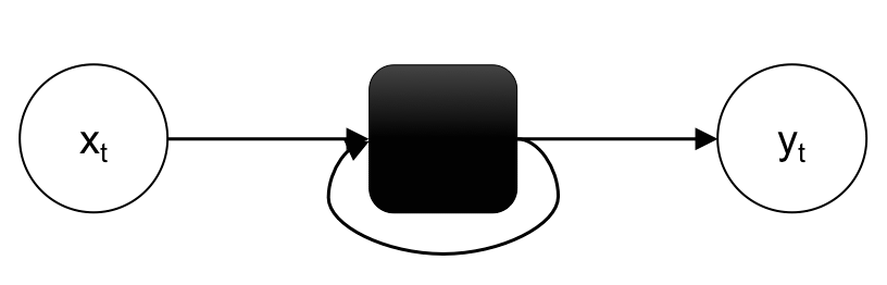*図1　RNN*

シーケンス型 … 複数の要素をまとめて扱える型
- リスト, タプル, 文字列 etc.

*An encoder network condenses an input sequence into a vector, and a decoder network unfolds that vector into a new sequence.*

エンコーダネットワークは入力シーケンスをベクトルに凝縮し、デコーダネットワークはそのベクトルを新しいシーケンスに展開する(図2)

図2 エンコーダ-デコーダネットワーク

エンコーダ … 入力を何かしらの（固定長）特徴ベクトルに変換する
- ここでは、入力文を単語の特徴量を並べたベクトルに変換する

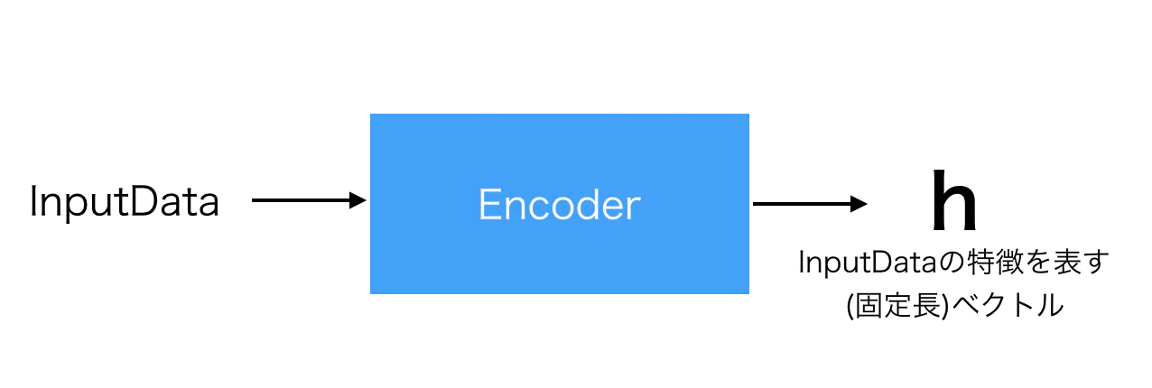
図3　InputDataを抽象的なベクトルにエンコード

デコーダ … Encoderでエンコードされた特徴ベクトルをデコードすることで何か新しいデータを生む
- OutputDataはInputDataと同じデータ形式である必要はない

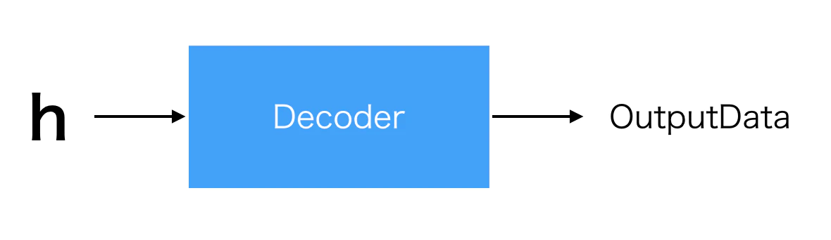
図4　特徴ベクトルをデコード

Encoder-Decoderモデル … エンコーダとデコーダをつなげたモデル
- 生成系のモデルであり、画像をテキストにしたり、音声からテキストを生成したり、日本語から英語（テキストから別のテキスト）に変換したりといった用途で用いられる

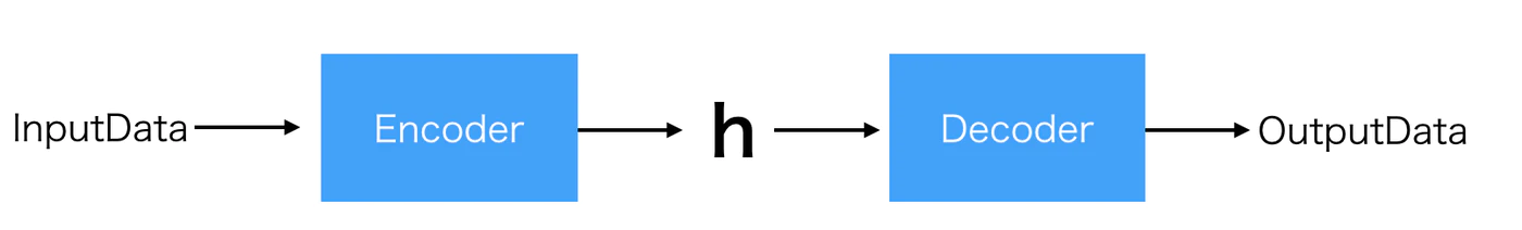
図5　Encoder-Decoderモデル

from __future__ import unicode_literals, print_function, division
# Python2 でも Python3 と同様にするためのインポート
# → ということは Python3　では必要ない？
from io import open
# これも Python3 には必要ないかも
import unicodedata
# Unicode のテキスト処理を行うため
import string
# 一般的な文字列操作
import re
# 正規表現操作
import random
# 乱数を生成

import torch
# torch基本モジュール
import torch.nn as nn
# ネットワーク構築用
from torch import optim
# SGDを使うため
import torch.nn.functional as F
# ネットワーク用関数

device = torch.device("cuda" if torch.cuda.is_available() else "cpu")

データファイルの読み込み

!unzip "data.zip"
# colab contentフォルダの直下に置く

!unzip "X.zip" … zipファイルを解凍

英語-日本語ペア辞書を作成

!unzip "jpn-eng.zip"

*図6 整理前の英語-日本語ペア*

with open("eng-jpn.txt", "w") as ej :
    ej.write("")
    # eng-jpn.txt を初期化

# eng-jpn.txt を data 直下に移動

with open(".txt", "w") … ファイルを開く
- withを使うことでブロック終了時に自動で閉じるため、close()を省略できる
- 第二引数
  - "r" … 読み取り
  - "w" … 書き込み（新規作成もしくは上書き）
    - ファイルが存在しなければ新規作成、存在していれば上書き（既存の内容は削除）で保存される
  - "a" … 追加書き込み
X.write("xyz") … ファイルXに文字列を書き込む

for line in open("jpn.txt", "r"):
    CC = re.findall("CC.*", line)
    # 一行ごとに帰属部分を抽出

    with open("eng-jpn.txt", "a") as ej :
        ej.write(line.replace(str(CC)[2:-2], ""))
        # 帰属部分を削除して eng-jpn.txt に追加書き込み
        # CC は list
        # そのまま str型にすると、 ["~~~~"] となる → スライサーを使用

for line in open() … open関数で開いたファイルが１行ずつfor文の変数に読み込まれ、最終行まで読み込み終わるとfor文が終了する
re.findall("X.*", line) … line内で"X.*"にマッチするすべての部分を文字列のリストとして返す
"X.*" … .は改行以外の任意の1文字、*は直前のパターンの0回以上の繰り返し
- Xから始まる部分を指定している
- "X.*y"とすれば、Xで始まりyで終わる部分を指定できる

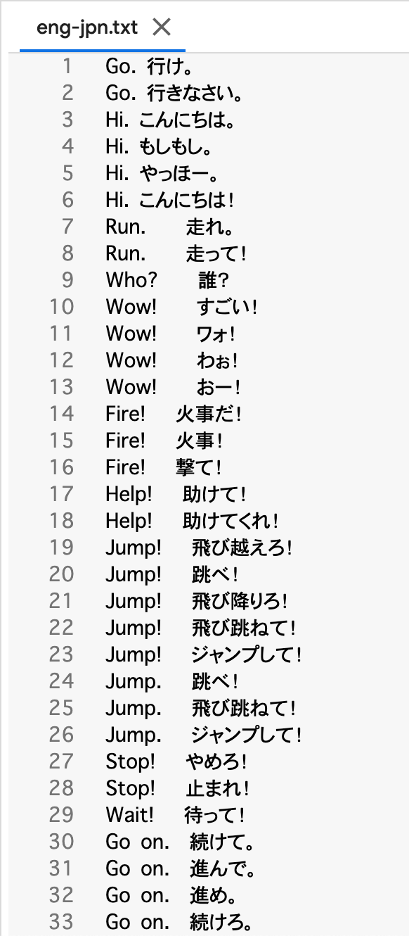*図7 整理した英語-日本語ペア*

データ準備

*Similar to the character encoding used in the character-level RNN tutorials, we will be representing each word in a language as a one-hot vector, or giant vector of zeros except for a single one (at the index of the word).*

文字レベルのRNNチュートリアルで使用されている文字エンコーディングと同様に、言語内の各単語をone-hotベクトル、つまり（単語のインデックスで）単一のベクトルを除いたゼロの巨大ベクトルとして表現する

*Compared to the dozens of characters that might exist in a language, there are many many more words, so the encoding vector is much larger.*

言語に存在する可能性のある数十の文字に比べて、さらに多くの単語があるため、エンコーディングベクトルははるかに大きくなる

*We will however cheat a bit and trim the data to only use a few thousand words per language.*

しかし、我々は少しごまかして、言語ごとに数千語しか使わないようにデータをトリミングする

図8　one-hotベクトル

*We’ll need a unique index per word to use as the inputs and targets of the networks later.*

後でネットワークの入力及びターゲットとして使用するためには、単語ごとに一意のインデックスが必要になる

*To keep track of all this we will use a helper class called Lang which has word → index (word2index) and index → word (index2word) dictionaries, as well as a count of each word word2count to use to later replace rare words.*

これらすべてを追跡するために、

単語 → インデックス(word2index)辞書
インデックス → 単語(index2word)辞書
各単語の数をカウントするword2count

これらを用いて珍しい単語を置き換える、Langと呼ばれるヘルパークラスを使用する

SOS_token = 0
EOS_token = 1

class Lang:
    def __init__(self, name):
        self.name = name
        # 登録する単語
        self.word2index = {}
        # 辞書を作成
        self.word2count = {}
        self.index2word = {0: "SOS", 1: "EOS"}
        # 0, 1番目はSOS, EOS
        self.n_words = 2
        # Count SOS and EOS

    def addSentence(self, sentence):
        for word in sentence.split(' '):
            # sentenceを空白で区切り単語化した中にwordがあった時
            self.addWord(word)

    def addWord(self, word):
        if word not in self.word2index:
        # もしwordが word2index辞書内にない場合
            self.word2index[word] = self.n_words
            # word を key としてその値に n_words をいれる
            self.word2count[word] = 1
            # word を key としてその値を1とする
            self.index2word[self.n_words] = word
            # n_words を key としてその値に word をいれる
            self.n_words += 1
        else:
        # wordが word2index辞書内にない場合
            self.word2count[word] += 1
            # word を key とした値に1を足す

SOS … Start of Statement
EOS … End of Statement

*The files are all in Unicode, to simplify we will turn Unicode characters to ASCII, make everything lowercase, and trim most punctuation.*

ファイルはすべてUnicodeで作成されている。簡単にするために、Unicode文字をASCIIに変換し、すべてを小文字にして、ほとんどの句読点を削除する

def unicodeToAscii(s):
# Unicode文字列をプレーンASCIIに変換する
    return ''.join(
        c for c in unicodedata.normalize('NFD', s)
        if unicodedata.category(c) != 'Mn')

def normalizeString(s):
# 全てを小文字にし、句読点などを削除する
    s = unicodeToAscii(s.lower().strip())
    s = re.sub(r"([.!?])", r" \1", s)
    s = re.sub(r"[^a-zA-Z.!?]+", r" ", s)
    return s

*To read the data file we will split the file into lines, and then split lines into pairs.*

データファイルを読み込むには、ファイルを行に分割してから、行をペアに分割する

*The files are all English → Other Language, so if we want to translate from Other Language → English I added the reverse flag to reverse the pairs.*

ファイルは全て英語 → 他言語であるから、他言語 → 英語で翻訳したい場合にはペアを逆にするために、逆フラグ(`reverse`)を追加した

def readLangs(lang1, lang2, reverse = False) :
    print("Reading lines...")

    # Read the file and split into lines
    # ファイルを読み込んで行に分割する
    lines = open('data/%s-%s.txt' % (lang1, lang2), encoding='utf-8').\
        read().strip().split('\n')
    # 'data/%s-%s.txt' % (lang1, lang2)
    # 一つ目の %s に　lang1, 二つ目の %s に lang2 を代入
    # "\n" は改行

    # Split every line into pairs and normalize
    # すべての行をペアに分割して正規化する
    pairs = [[normalizeString(s) for s in l.split('\t')] for l in lines]
    # "\t" はタブ

    # Reverse pairs, make Lang instances
    # ペアを反転させ、Langインスタンスを作る
    if reverse:
    # もし reverse = False なら
        pairs = [list(reversed(p)) for p in pairs]
        # ペアを反転する
        input_lang = Lang(lang2)
        output_lang = Lang(lang1)
    else:
        input_lang = Lang(lang1)
        output_lang = Lang(lang2)

    return input_lang, output_lang, pairs

*Since there are a lot of example sentences and we want to train something quickly, we’ll trim the data set to only relatively short and simple sentences.*

たくさんの例文があるが、素早く学習するために比較的短くてシンプルな文だけが残るようににデータセットをトリミングする

*Here the maximum length is 10 words (that includes ending punctuation) and we’re filtering to sentences that translate to the form “I am” or “He is” etc. (accounting for apostrophes replaced earlier).*

ここでは、最大の長さは10語（語尾の句読点を含む）で、"I am" や "He is" などの形に翻訳された文にフィルタリングしている（以前に置き換えられたアポストロフィを考慮する）

アポストロフィ … I'm, he's 等の '

MAX_LENGTH = 10

eng_prefixes = (
    "i am ", "i m ",
    "he is", "he s ",
    "she is", "she s ",
    "you are", "you re ",
    "we are", "we re ",
    "they are", "they re "
)

def filterPair(p):
    return len(p[0].split(' ')) < MAX_LENGTH and \
        len(p[1].split(' ')) < MAX_LENGTH and \
        p[1].startswith(eng_prefixes)

def filterPairs(pairs):
    return [pair for pair in pairs if filterPair(pair)]

\ … 文末に入力するとその後の改行を無視する
- 一行が長くなる時に利用する
X.startswith("あ") … 文字列Xがあから始まっているときTrueを返し、そうでないときFalseを返す

*The full process for preparing the data is:*

データを準備するための完全なプロセスは次のとおり

Read text file and split into lines, split lines into pairs
- テキストファイルを読み取り、行に分割、行をペアに分割
Normalize text, filter by length and content
- テキストファイルを読み取り、行に分割、行をペアに分割
Make word lists from sentences in pairs
- ペアの文章から単語リストを作成する

def prepareData(lang1, lang2, reverse=False):
    input_lang, output_lang, pairs = readLangs(lang1, lang2, reverse)
    print("Read %s sentence pairs" % len(pairs))
    pairs = filterPairs(pairs)
    print("Trimmed to %s sentence pairs" % len(pairs))
    print("Counting words...")
    for pair in pairs:
        input_lang.addSentence(pair[0])
        output_lang.addSentence(pair[1])
        # addSentence() は空白区切りで単語を認識
        # 日本語では空白で単語を区切ることができない！！！！
    print("Counted words:")
    print(input_lang.name, input_lang.n_words)
    print(output_lang.name, output_lang.n_words)
    return input_lang, output_lang, pairs

input_lang, output_lang, pairs = prepareData('eng', 'fra', True)
print(random.choice(pairs))

Out

Reading lines...
Read 135842 sentence pairs
Trimmed to 10599 sentence pairs
Counting words...
Counted words:
fra 4345
eng 2803
['je vais me marier en octobre .', 'i m getting married in october .']

Seq2Seqモデル

*A Recurrent Neural Network, or RNN, is a network that operates on a sequence and uses its own output as input for subsequent steps.*

再帰型ニューラルネットワーク（RNN）は、シーケンス上で動作し、自身の出力をその後のステップの入力として使用するネットワーク

*A Sequence to Sequence network, or seq2seq network, or Encoder Decoder network, is a model consisting of two RNNs called the encoder and decoder.*

Sequence to Sequenceネットワーク(seq2seqネットワーク、エンコーダデコーダネットワークとも言う)は、エンコーダとデコーダと呼ばれる2つのRNNで構成されるモデルである。

*The encoder reads an input sequence and outputs a single vector, and the decoder reads that vector to produce an output sequence.*

エンコーダは入力シーケンスを読み込んで単一のベクトルを出力し、デコーダはそのベクトルを読み取って出力シーケンスを生成する

図2・再

*Unlike sequence prediction with a single RNN, where every input corresponds to an output, the seq2seq model frees us from sequence length and order, which makes it ideal for translation between two languages.*

すべての入力が出力に対応する単一のRNNによるシーケンス予測とは異なり、seq2seqモデルはシーケンスの長さや順序から解放されるので、2つの言語間の翻訳に最適である

*Consider the sentence “Je ne suis pas le chat noir” → “I am not the black cat”.*

「Je ne suis pas le chat noir」→「I am not the black cat」という文について考える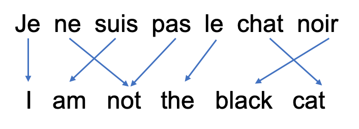

*図9　仏英簡易対応「私は黒猫ではありません」*

*Most of the words in the input sentence have a direct translation in the output sentence, but are in slightly different orders, e.g. “chat noir” and “black cat”.*

入力文のほとんどの単語は出力文で直訳されているが、「chat noir」と「black cat」のように少し順番が違うものもある

*Because of the “ne/pas” construction there is also one more word in the input sentence.*

「ne / pas」の構造のため、入力文の単語数は一つ多くなる

ne/pas構造 … フランス語の否定文における決まり
- 否定文の動詞をneとpasで挟まなくてはいけない

*It would be difficult to produce a correct translation directly from the sequence of input words.*

入力された単語の並びから直接正しい翻訳を作成するのは困難である

*With a seq2seq model the encoder creates a single vector which, in the ideal case, encodes the “meaning” of the input sequence into a single vector — a single point in some N dimensional space of sentences.*

seq2seqモデルでは、エンコーダが一つのベクトルを作成し、理想的なケースでは、入力シーケンスの「意味」を単一のベクトル（文のN次元空間の単一の点）にエンコードする

エンコーダ

*The encoder of a seq2seq network is a RNN that outputs some value for every word from the input sentence.*

seq2seqネットワークのエンコーダは、入力文の各単語に対して何らかの値を出力するRNNである

*For every input word the encoder outputs a vector and a hidden state, and uses the hidden state for the next input word.*

各入力語に対して、エンコーダはベクトルと隱れ状態（中間出力）を出力し、次の入力語としてその隱れ状態を使用する

隱れ状態(中間出力) … 当該時刻 $t$ の時系列情報 $x_t$ と前時刻 $t-1$ の隠れ状態 $h_{t−1}$ を組み合わせて活性化したもの

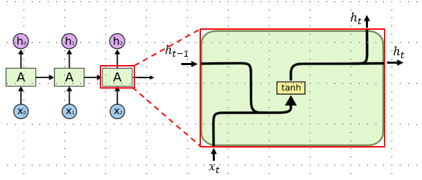*図10　エンコーダ内部*

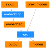
図11　エンコーダネットワーク

class EncoderRNN(nn.Module):
    def __init__(self, input_size, hidden_size):
        super(EncoderRNN, self).__init__()
        self.hidden_size = hidden_size

        self.embedding = nn.Embedding(input_size, hidden_size)
        # 行が各単語ベクトル、列が埋め込みの次元である行列を生成
        # Embedding(扱う単語の数, 隱れ層のサイズ(埋め込みの次元))
        self.gru = nn.GRU(hidden_size, hidden_size)

    def forward(self, input, hidden):
        embedded = self.embedding(input).view(1, 1, -1)
        # 1 x 1 x n 型にベクトルサイズを変える
        # n の値は自動的に設定される
        output = embedded
        output, hidden = self.gru(output, hidden)
        return output, hidden
        # output が各系列のGRUの隱れ層ベクトル

    def initHidden(self):
        return torch.zeros(1, 1, self.hidden_size, device=device)

Embedding … 埋め込み
- 文や単語、文字など自然言語の構成要素に対して、何らかの空間におけるベクトルを与えること
GRU … 多層ゲート型再発ユニット(Gated Recurrent Unit)
- LSTMの忘却ゲートと入力ゲートを単一の更新ゲートにマージし隠れ状態のみを伝達していくニューラルネットワークのモデル

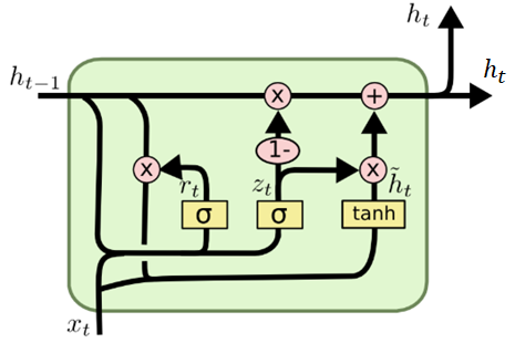*図12　GRU内部*

デコーダ

*The decoder is another RNN that takes the encoder output vector(s) and outputs a sequence of words to create the translation.*

デコーダは、エンコーダの出力ベクトルを受け取り、一連の単語を出力して翻訳を作成するもう一つのRNN

シンプルなデコーダ

*In the simplest seq2seq decoder we use only last output of the encoder.*

最も単純なseq2seqデコーダでは、エンコーダの最後の出力のみを使用する

*This last output is sometimes called the context vector as it encodes context from the entire sequence.*

この最後の出力は、シーケンス全体のコンテキストをエンコードするので、**コンテキストベクトル**と呼ばれることもある

*This context vector is used as the initial hidden state of the decoder.*

このコンテキストベクトルは、デコーダの初期の隠れ状態として使われる

*At every step of decoding, the decoder is given an input token and hidden state.*

デコードの各ステップで、デコーダには入力トークンと隠れ状態が与えられる

*The initial input token is the start-of-string token, and the first hidden state is the context vector (the encoder’s last hidden state).*

最初の入力トークンは、文字列開始の``トークンであり、最初の隠れ状態は、コンテキストベクトル（エンコーダの最後の隠れ状態）である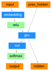

図13　シンプルデコーダネットワーク

class DecoderRNN(nn.Module):
    def __init__(self, hidden_size, output_size):
        super(DecoderRNN, self).__init__()
        self.hidden_size = hidden_size

        self.embedding = nn.Embedding(output_size, hidden_size)
        self.gru = nn.GRU(hidden_size, hidden_size)
        self.out = nn.Linear(hidden_size, output_size)
        self.softmax = nn.LogSoftmax(dim=1)

    def forward(self, input, hidden):
        output = self.embedding(input).view(1, 1, -1)
        output = F.relu(output)
        output, hidden = self.gru(output, hidden)
        output = self.softmax(self.out(output[0]))
        return output, hidden

    def initHidden(self):
        return torch.zeros(1, 1, self.hidden_size, device=device)

softmax … 非線形関数の1つであり、実数値ベクトルの入力に対して確率分布を返す
- dim … NumPyのaxisと同じ働き。軸を定める
  - 行方向がdim=0、列方向がdim=1となり、3次元になった場合は奥行き方向がdim=2である
.relu() … 入力が負のときは0、正のときはそのまま入力を出力するユニット

*I encourage you to train and observe the results of this model, but to save space we’ll be going straight for the gold and introducing the Attention Mechanism.*

このモデルの結果を訓練して観察することをお勧めするが、スペースを節約するために、最も有効なアテンションメカニズムを導入する

Attentionデコーダ

*If only the context vector is passed betweeen the encoder and decoder, that single vector carries the burden of encoding the entire sentence.*

エンコーダとデコーダの間にコンテキストベクトルだけが渡される場合、その単一のベクトルが文全体をエンコードする負担を負うことになる

*Attention allows the decoder network to “focus” on a different part of the encoder’s outputs for every step of the decoder’s own outputs.*

`Attention`により、デコーダネットワークはデコーダ自身の出力のステップごとに、エンコーダの出力の異なる部分に**フォーカス**することができる

Encoder側の各隠れ層の値をすべてDecoder側の各層に渡す
- Encoder側の隠れ層ベクトルの数は、Encoder側のインプットとなる系列の長さに依存するので、系列の長さを考慮した形になっている
Decoder側の各層において、Encoder側から渡された各隠れ層のベクトルのうち、最も注意すべきベクトルを選び出して(→フォーカス)特徴に加える
- 選び出すという操作は微分できないが、各要素のどこに注意すべきかをsoftmaxで確率的に重み付けした形で選ぶ操作を行う

*First we calculate a set of attention weights.*

まず、`Attention`の重みのセットを計算する

*These will be multiplied by the encoder output vectors to create a weighted combination.*

これらをエンコーダの出力ベクトルで乗算して、重み付けされた組み合わせを作成する

*The result (called attn_applied in the code) should contain information about that specific part of the input sequence, and thus help the decoder choose the right output words.*

その結果（`attn_applied`コードで呼び出される）には入力シーケンスのその特定の部分に関する情報が含まれているため、デコーダが正しい出力語を選択するのに役立つ

図14　Attentionデコーダネットワーク

*Calculating the attention weights is done with another feed-forward layer attn, using the decoder’s input and hidden state as inputs.*

`Attention`の重みの計算は、デコーダの入力と隠れ状態を入力として使用する別のフィードフォワード層`attn`で行われる

フィードフォワード層 … データの流れが一方向であって、データが行ったり来たり、あるいはループしたりしないような層

*Because there are sentences of all sizes in the training data, to actually create and train this layer we have to choose a maximum sentence length (input length, for encoder outputs) that it can apply to.*

学習データにはあらゆるサイズの文が含まれているため、実際にこのレイヤーを作成して学習するには、このレイヤーが適用できる最大文長（エンコーダの出力の入力長）を選択しなければならない

*Sentences of the maximum length will use all the attention weights, while shorter sentences will only use the first few.*

最大長の文はすべての`Attention`の重みを使用するが、短い文の場合は最初の数文のみを使用する

Attention の処理の流れ

ここではEncoder側のインプットの系列が$w1, w2, w3$の3つのとき、Decoder側が $w'1, w'2$の2つのケースを扱う

Encoder側の各隠れ層の値をそれぞれ$h_1, h_2, ⋯, h_n$ としたとき、$hs=[h_1,h_2,⋯,h_n]$をDecoder側の各層に渡す。

図15　$1.$
Decoder側の各隠れ層のベクトル(ここでは$d_i$とする)と$hs$の各ベクトル$h_1,h_2,⋯$との内積を計算する。これはDecoder側の各ベクトルと$hs$の各ベクトルがどれだけ似ているかを計算していることを意味する（内積は(**$,$**)で表記）

図16　$2.$
$2.$で計算した内積をsoftmaxで確率表現に変換する（これがattn_weights）

図17　$3.$
$hs$の各要素をattn_weightsで重み付けし、全部を足しあわせて1本のベクトル（コンテキストベクトル）とする

図18　$4.$
コンテキストベクトルと$d_i$を結合して、1本のベクトルにする

図19　$5.$

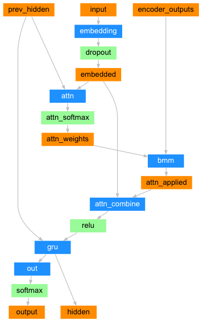
図20　Attentionデコーダネットワーク

class AttnDecoderRNN(nn.Module):
    def __init__(self, hidden_size, output_size, dropout_p=0.1, max_length=MAX_LENGTH):
        super(AttnDecoderRNN, self).__init__()
        self.hidden_size = hidden_size
        self.output_size = output_size
        self.dropout_p = dropout_p
        self.max_length = max_length

        self.embedding = nn.Embedding(self.output_size, self.hidden_size)
        self.attn = nn.Linear(self.hidden_size * 2, self.max_length)
        self.attn_combine = nn.Linear(self.hidden_size * 2, self.hidden_size)
        # 線形結合を計算
        # hidden_size * 2
        # → 各系列のGRUの隠れ層とAttention層で計算したコンテキストベクトルをtorch.catでつなぎ合わせることで長さが２倍になる
        self.dropout = nn.Dropout(self.dropout_p)
        # 過学習の回避
        self.gru = nn.GRU(self.hidden_size, self.hidden_size)
        self.out = nn.Linear(self.hidden_size, self.output_size)

    def forward(self, input, hidden, encoder_outputs):
        embedded = self.embedding(input).view(1, 1, -1)
        embedded = self.dropout(embedded)

        attn_weights = F.softmax(
            self.attn(torch.cat((embedded[0], hidden[0]), 1)), dim=1)
        # 列方向を確率変換したいから dim = 1
        attn_applied = torch.bmm(attn_weights.unsqueeze(0),
                                 encoder_outputs.unsqueeze(0))
        # bmm でバッチも考慮してまとめて行列計算
        # ここでバッチが考慮されるから unsqueeze(0) が必要

        output = torch.cat((embedded[0], attn_applied[0]), 1)
        output = self.attn_combine(output).unsqueeze(0)

        output = F.relu(output)
        output, hidden = self.gru(output, hidden)

        output = F.log_softmax(self.out(output[0]), dim=1)
        return output, hidden, attn_weights

    def initHidden(self):
    # コンテキストベクトルをまとめるための入れ物を用意する
        return torch.zeros(1, 1, self.hidden_size, device=device)

torch.cat([x1, x2]) … torch.Tensorをリストに入れて渡すと、それらを連結したTensorを返す
- 連結する軸はdimによって指定する
.unsqueeze(0) … バッチサイズを追加する

*There are other forms of attention that work around the length limitation by using a relative position approach. Read about “local attention” in Effective Approaches to Attention-based Neural Machine Translation.*

相対位置アプローチを使用して長さ制限を回避する`Attention`の他の形態がある。詳しくは[Effective Approaches to Attention-based Neural Machine Translation](https://arxiv.org/abs/1508.04025) > "local attention"

学習

学習データの準備

*To train, for each pair we will need an input tensor (indexes of the words in the input sentence) and target tensor (indexes of the words in the target sentence).*

学習するには、各ペアについて、入力テンソル（入力文に含まれる単語のインデックス）とターゲットテンソル（ターゲット文に含まれる単語のインデックス）が必要である

*While creating these vectors we will append the EOS token to both sequences.*

これらのベクトルを作成する際に、`EOSトークン`を両方のシーケンスに追加する

def indexesFromSentence(lang, sentence):
    return [lang.word2index[word] for word in sentence.split(' ')]

def tensorFromSentence(lang, sentence):
    indexes = indexesFromSentence(lang, sentence)
    indexes.append(EOS_token)
    return torch.tensor(indexes, dtype=torch.long, device=device).view(-1, 1)

def tensorsFromPair(pair):
    input_tensor = tensorFromSentence(input_lang, pair[0])
    target_tensor = tensorFromSentence(output_lang, pair[1])
    return (input_tensor, target_tensor)

モデルのトレーニング

*To train we run the input sentence through the encoder, and keep track of every output and the latest hidden state.*

訓練するには、入力文をエンコーダを通して実行し、すべての出力と最新の隠れ状態を追跡する

*Then the decoder is given the token as its first input, and the last hidden state of the encoder as its first hidden state.*

デコーダには最初の入力として`トークン`が与えられ、最初の隠れ状態としてエンコーダの最後の隠れ状態が与えられる

*“Teacher forcing” is the concept of using the real target outputs as each next input, instead of using the decoder’s guess as the next input.*

「教師強制」とは、デコーダの推測を次の入力として使用する代わりに、実際のターゲット出力を次の各入力として使用するという概念

*Using teacher forcing causes it to converge faster but when the trained network is exploited, it may exhibit instability.*

教師強制を使用すると収束がより速くなるが、訓練されたネットワークが悪用されると不安定になることがある

*You can observe outputs of teacher-forced networks that read with coherent grammar but wander far from the correct translation - intuitively it has learned to represent the output grammar and can “pick up” the meaning once the teacher tells it the first few words, but it has not properly learned how to create the sentence from the translation in the first place.*

一貫した文法で翻訳するが、正しい翻訳とはかけ離れた教師強制ネットワークの出力を観察することができる。これは、直感的には出力された文法を表現することを学習し、教師が最初の数語を教えれば意味を**ピックアップ**できるが、そもそも翻訳から文を作成する方法を正しく学習していないからである

*Because of the freedom PyTorch’s autograd gives us, we can randomly choose to use teacher forcing or not with a simple if statement.*

PyTorchの`autograd`が与えてくれる自由度のおかげで、単純なif文で教師強制を使うか使わないかをランダムに選択することができる

*Turn teacher_forcing_ratio up to use more of it.*

`teacher_forcing_ratio`を上げると教師強制の使用回数を増やす

teacher_forcing_ratio = 0.5

def train(input_tensor, target_tensor, encoder, decoder, encoder_optimizer, decoder_optimizer, criterion, max_length=MAX_LENGTH):
    encoder_hidden = encoder.initHidden()

    encoder_optimizer.zero_grad()
    decoder_optimizer.zero_grad()
    # 勾配の初期化

    input_length = input_tensor.size(0)
    target_length = target_tensor.size(0)
    # データをテンソルに変換する

    encoder_outputs = torch.zeros(max_length, encoder.hidden_size, device=device)

    loss = 0

    for ei in range(input_length):
        encoder_output, encoder_hidden = encoder(
            input_tensor[ei], encoder_hidden)
        encoder_outputs[ei] = encoder_output[0, 0]

    decoder_input = torch.tensor([[SOS_token]], device=device)

    decoder_hidden = encoder_hidden

    use_teacher_forcing = True if random.random() < teacher_forcing_ratio else False

    if use_teacher_forcing:
    # 教師強制を使用する場合
        # Teacher forcing: Feed the target as the next input
        # 教師強制 : 次の入力としてターゲットを送る
        for di in range(target_length):
            decoder_output, decoder_hidden, decoder_attention = decoder(
                decoder_input, decoder_hidden, encoder_outputs)
            loss += criterion(decoder_output, target_tensor[di])
            decoder_input = target_tensor[di]

    else:
        # Without teacher forcing: use its own predictions as the next input
        # 教師強制の使用をしない : 次の入力として独自の予測値を使用する
        for di in range(target_length):
            decoder_output, decoder_hidden, decoder_attention = decoder(
                decoder_input, decoder_hidden, encoder_outputs)
            topv, topi = decoder_output.topk(1)
            decoder_input = topi.squeeze().detach()  # detach from history as input

            loss += criterion(decoder_output, target_tensor[di])
            if decoder_input.item() == EOS_token:
                break

    loss.backward()
    # 誤差逆伝播

    encoder_optimizer.step()
    decoder_optimizer.step()
    # パラメータの更新

    return loss.item() / target_length

*This is a helper function to print time elapsed and estimated time remaining given the current time and progress %.*

現在の時刻と進行度をパーセンテージとして、与えられた経過時間と推定残り時間を表示するヘルパー関数

import time
import math

def asMinutes(s):
    m = math.floor(s / 60)
    s -= m * 60
    return '%dm %ds' % (m, s)

def timeSince(since, percent):
    now = time.time()
    s = now - since
    es = s / (percent)
    rs = es - s
    return '%s (- %s)' % (asMinutes(s), asMinutes(rs))

*The whole training process looks like this:*

トレーニング全体の流れは以下の通り

Start a timer
- タイマーを開始する
Initialize optimizers and criterion
- オプティマイザと基準を初期化する
  - オプティマイザ … 最適化
Create set of training pairs
- トレーニングペアのセットを作成
Start empty losses array for plotting
- プロットのために空の損失配列を開始する

*Then we call train many times and occasionally print the progress (% of examples, time so far, estimated time) and average loss.*

そして何度も`terain`を呼び出して、時々進捗状況（例の％、これまでの時間、推定時間）と平均損失を表示する

def trainIters(encoder, decoder, n_iters, print_every=1000, plot_every=100, learning_rate=0.01):
    start = time.time()
    plot_losses = []
    print_loss_total = 0
    # Reset every print_every
    # print_every ごとにリセットする
    plot_loss_total = 0
    # Reset every plot_every
    # plot_every ごとにリセットする

    encoder_optimizer = optim.SGD(encoder.parameters(), lr=learning_rate)
    decoder_optimizer = optim.SGD(decoder.parameters(), lr=learning_rate)
    # 最適化

    training_pairs = [tensorsFromPair(random.choice(pairs))
                      for i in range(n_iters)]
                      
    criterion = nn.NLLLoss()
    # 損失関数

    for iter in range(1, n_iters + 1):
        training_pair = training_pairs[iter - 1]
        input_tensor = training_pair[0]
        target_tensor = training_pair[1]

        loss = train(input_tensor, target_tensor, encoder,
                     decoder, encoder_optimizer, decoder_optimizer, criterion)
        print_loss_total += loss
        plot_loss_total += loss

        if iter % print_every == 0:
            print_loss_avg = print_loss_total / print_every
            print_loss_total = 0
            print('%s (%d %d%%) %.4f' % (timeSince(start, iter / n_iters),
                                         iter, iter / n_iters * 100, print_loss_avg))

        if iter % plot_every == 0:
            plot_loss_avg = plot_loss_total / plot_every
            plot_losses.append(plot_loss_avg)
            plot_loss_total = 0

    showPlot(plot_losses)

結果のプロット

*Plotting is done with matplotlib, using the array of loss values plot_losses saved while training.*

学習中に保存された損失値の配列`plot_losses`を用いて、`matplotlib`てプロットされる

import matplotlib.pyplot as plt
plt.switch_backend('agg')
import matplotlib.ticker as ticker
import numpy as np

def showPlot(points):
    plt.figure()
    fig, ax = plt.subplots()
    loc = ticker.MultipleLocator(base=0.2)
    # this locator puts ticks at regular intervals
    # loc は定期的に ticker を配置する
    ax.yaxis.set_major_locator(loc)
    plt.plot(points)
    plt.savefig("plot.png")
    # content フォルダ下に保存される

評価

*Evaluation is mostly the same as training, but there are no targets so we simply feed the decoder’s predictions back to itself for each step.*

評価はトレーニングとほとんど同じであるが、ターゲットがないため、各ステップごとにデコーダの予測値を自分自身にフィードバックする

*Every time it predicts a word we add it to the output string, and if it predicts the EOS token we stop there.*

デコーダが単語を予測するたびに出力文字列に追加し、EOSトークンを予測した場合はそこで停止する

*We also store the decoder’s attention outputs for display later.*

また、後で表示するためにデコーダの`Attention`出力も保存する

def evaluate(encoder, decoder, sentence, max_length=MAX_LENGTH):
    with torch.no_grad():
        input_tensor = tensorFromSentence(input_lang, sentence)
        input_length = input_tensor.size()[0]
        encoder_hidden = encoder.initHidden()

        encoder_outputs = torch.zeros(max_length, encoder.hidden_size, device=device)

        for ei in range(input_length):
            encoder_output, encoder_hidden = encoder(input_tensor[ei],
                                                     encoder_hidden)
            encoder_outputs[ei] += encoder_output[0, 0]

        decoder_input = torch.tensor([[SOS_token]], device=device)  
        # SOS

        decoder_hidden = encoder_hidden

        decoded_words = []
        decoder_attentions = torch.zeros(max_length, max_length)

        for di in range(max_length):
            decoder_output, decoder_hidden, decoder_attention = decoder(
                decoder_input, decoder_hidden, encoder_outputs)
            decoder_attentions[di] = decoder_attention.data
            topv, topi = decoder_output.data.topk(1)
            if topi.item() == EOS_token:
                decoded_words.append('<EOS>')
                break
            else:
                decoded_words.append(output_lang.index2word[topi.item()])

            decoder_input = topi.squeeze().detach()

        return decoded_words, decoder_attentions[:di + 1]

*We can evaluate random sentences from the training set and print out the input, target, and output to make some subjective quality judgements:*

トレーニングセットからランダムな文章を評価し、入力、ターゲット、出力を`print`することで、主観的な品質判断を行うことができる

def evaluateRandomly(encoder, decoder, n=10):
    for i in range(n):
        pair = random.choice(pairs)
        print('>', pair[0])
        print('=', pair[1])
        output_words, attentions = evaluate(encoder, decoder, pair[0])
        output_sentence = ' '.join(output_words)
        print('<', output_sentence)
        print('')

トレーニングと評価

*With all these helper functions in place (it looks like extra work, but it makes it easier to run multiple experiments) we can actually initialize a network and start training.*

これらのヘルパー関数を全て配置すると（余計な作業のように見えるが、複数の実験を行うのが簡単になる）、実際にネットワークを初期化して学習を開始することができる

*Remember that the input sentences were heavily filtered.*

入力文は大きくフィルタリングされている

*For this small dataset we can use relatively small networks of 256 hidden nodes and a single GRU layer.*

この小さなデータセットでは、256個の隠れノードと1つのGRU層からなる比較的小さなネットワークを使うことができる

*After about 40 minutes on a MacBook CPU we’ll get some reasonable results.*

MacBookのCPUで約40分後には、それなりの結果が得られるだろう　→　Colab GPU上で約20分

*If you run this notebook you can train, interrupt the kernel, evaluate, and continue training later.*

このノートを実行すると、トレーニングをしたり、カーネルを中断したり、評価したり、後でトレーニングを続けたりすることができる

*Comment out the lines where the encoder and decoder are initialized and run trainIters again.*

**エンコーダとデコーダが初期化されている行をコメントアウト**して、再度`trainIters`を実行すれば良い

hidden_size = 256
encoder1 = EncoderRNN(input_lang.n_words, hidden_size).to(device)
attn_decoder1 = AttnDecoderRNN(hidden_size, output_lang.n_words, dropout_p=0.1).to(device)

trainIters(encoder1, attn_decoder1, 75000, print_every=5000)

図21　[plot.png]損失率のグラフ

Out

1m 26s (- 20m 9s) (5000 6%) 2.8497
2m 50s (- 18m 25s) (10000 13%) 2.2986
4m 13s (- 16m 53s) (15000 20%) 1.9580
5m 37s (- 15m 28s) (20000 26%) 1.7055
7m 2s (- 14m 5s) (25000 33%) 1.5105
8m 27s (- 12m 40s) (30000 40%) 1.3366
9m 50s (- 11m 14s) (35000 46%) 1.2163
11m 12s (- 9m 48s) (40000 53%) 1.0983
12m 35s (- 8m 23s) (45000 60%) 0.9884
13m 58s (- 6m 59s) (50000 66%) 0.9022
15m 21s (- 5m 35s) (55000 73%) 0.7916
16m 44s (- 4m 11s) (60000 80%) 0.7510
18m 7s (- 2m 47s) (65000 86%) 0.6791
19m 31s (- 1m 23s) (70000 93%) 0.6039
20m 53s (- 0m 0s) (75000 100%) 0.5575

evaluateRandomly(encoder1, attn_decoder1)

Out

> je n abandonne pas si facilement .
= i m no quitter .
< i m no quitter . <EOS>

> je vais me coucher !
= i m going to bed .
< i m going to bed . <EOS>

> elle est gracieuse .
= she is graceful .
< she is graceful . <EOS>

> vous etes invitee .
= you re invited .
< you re invited . <EOS>

> nous ne sommes pas contents .
= we re not happy .
< we re not happy . <EOS>

> vous etes plus grands que moi .
= you re taller than i am .
< you re taller than i am . <EOS>

> je suis plus beau que tom .
= i m better looking than tom .
< i m more looking than tom . <EOS>

> tu dramatises .
= you re overreacting .
< you re overreacting . <EOS>

> il est cale en litterature anglaise .
= he is well read in english literature .
< he is well acquainted in his . . <EOS>

> je suis ici n est ce pas ?
= i m here aren t i ?
< i m here aren t you ? <EOS>

Attention の視覚化

*A useful property of the attention mechanism is its highly interpretable outputs.*

Attentionメカニズムの有用な特性は、その高度に解釈可能な出力である

*Because it is used to weight specific encoder outputs of the input sequence, we can imagine looking where the network is focused most at each time step.*

これは入力シーケンスの特定のエンコーダ出力の重み付けに使用されるため、各タイムステップでネットワークが最も集中している場所を見ることが想像できる

*You could simply run plt.matshow(attentions) to see attention output displayed as a matrix, with the columns being input steps and rows being output steps:*

単純に`plt.matshow(attentions)`を実行すると、Attention出力が行列として表示され、このとき列が入力ステップ、行が出力ステップとなる

output_words, attentions = evaluate(
    encoder1, attn_decoder1, "je suis trop froid .")
plt.matshow(attentions.numpy())

plt.savefig("matshow.png")

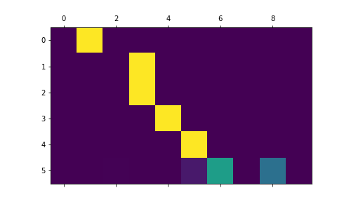
図22　[matshow.png]

*For a better viewing experience we will do the extra work of adding axes and labels:*

より見やすくするために、軸とラベルの追加作業を行う

def showAttention(input_sentence, output_words, attentions):
    # Set up figure with colorbar
    fig = plt.figure()
    ax = fig.add_subplot(111)
    cax = ax.matshow(attentions.numpy(), cmap='bone')
    fig.colorbar(cax)

    # Set up axes
    ax.set_xticklabels([''] + input_sentence.split(' ') +
                       ['<EOS>'], rotation=90)
    ax.set_yticklabels([''] + output_words)

    # Show label at every tick
    ax.xaxis.set_major_locator(ticker.MultipleLocator(1))
    ax.yaxis.set_major_locator(ticker.MultipleLocator(1))

    plt.savefig("matshows1.png")


def evaluateAndShowAttention(input_sentence):
    output_words, attentions = evaluate(
        encoder1, attn_decoder1, input_sentence)
    print('input =', input_sentence)
    print('output =', ' '.join(output_words))
    showAttention(input_sentence, output_words, attentions)


evaluateAndShowAttention("elle a cinq ans de moins que moi .")

#evaluateAndShowAttention("elle est trop petit .")

#evaluateAndShowAttention("je ne crains pas de mourir .")

#evaluateAndShowAttention("c est un jeune directeur plein de talent .")

# 一つずつやらないと上書き保存される
# plt.savefig() の名前を変更して順に実行する

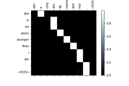
図22　[matshows1.png]

図23　[matshows2.png]

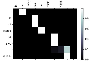
図24　[matshows3.png]

図25　[matshows4.png]

Out

input = elle a cinq ans de moins que moi .
output = she is six years younger than i am . <EOS>
input = elle est trop petit .
output = she s too short . <EOS>
input = je ne crains pas de mourir .
output = i m not scared of dying . <EOS>
input = c est un jeune directeur plein de talent .
output = he is a dumb young of guy . <EOS>

参考文献

You get articles that match your needs
You can efficiently read back useful information
You can use dark theme

What you can do with signing up