はじめに
前半でROC、後半でFROCについて書いています。
ROC曲線
ROC曲線(Receiver Operating Characteristic Curve)は、二値分類モデルの精度を測ることができる最もポピュラーな解析手法の1つです。
ROC曲線は、左肩が左上に上がるほどよいと覚えておくと便利です。
この性質を知っていれば、モデルの精度比較などを行う際にひと目で大まかなモデル間の分類精度を把握することができます。
この曲線から、曲線下面積(AUC:Area Under Curve, Area Under the Receiver Operating Characteristic Curve (ROC AUC) )という客観的な分類精度の指標を得ることもできます。
ROC曲線の例(scikit-learnのチュートリアル)を引用させていただきます。
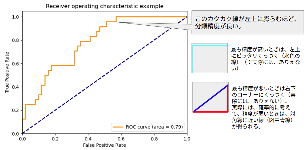
(リンク:https://scikit-learn.org/stable/auto_examples/model_selection/plot_roc.html)
ROC曲線の描き方
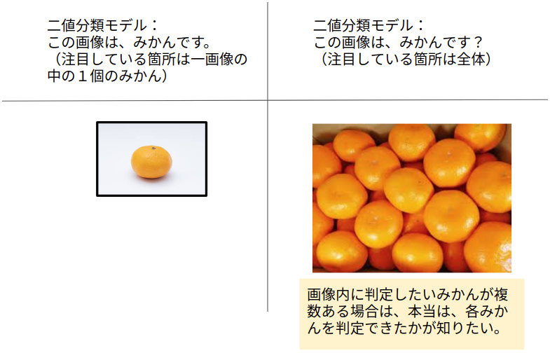
例えば、画像からみかんを識別する分類モデルを作ったとします。
この分類モデルはみかんか、みかんでないかを(一般的な精度で)予測できたとします。
そして、このモデルの精度をROC曲線で確認してみなければならない状況になったとします。
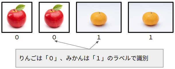
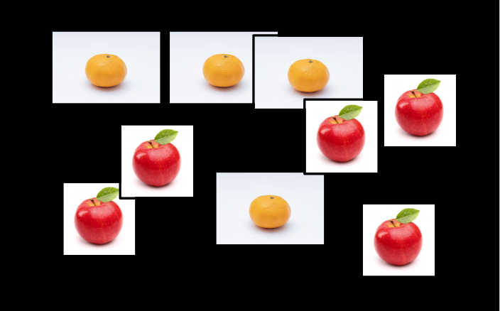
モデルの精度のテストには、りんごとみかんの画像を用いることとします。
りんごとみかんの画像はそれぞれ2枚ずつあるとしましょう。
左から、りんご1号、りんご2号、みかん1号、みかん2号です。
このようなテストをするときは、機械が処理しやすいように画像の種類ごとにラベルを設けます。
このモデルは、みかんか、そうでないかを予測しますから、りんごは0、みかんは1とラベルします(画像は同じですが、1号と2号は違うものと想像して下さい)。
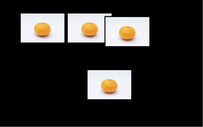
そして、分類モデルに、りんご1号、りんご2号、みかん1号、みかん2号の順で分類予測させたとします。
このときの正解ラベルは、[0, 0, 1, 1]になります。
これは、りんごラベルは0、みかんラベルは1であるので、画像の入力の順に合わせて、このような正解ラベルになるというわけです。
では実際にモデルに画像を予測させてみたとします。
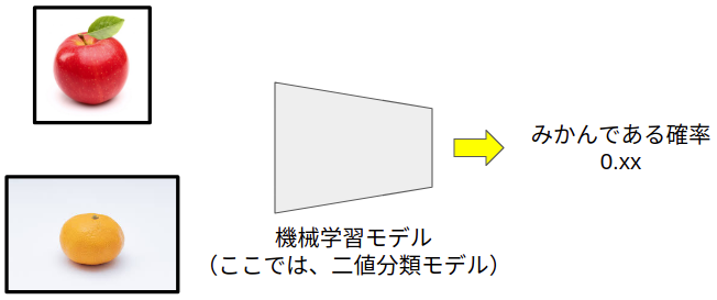
上図の0.xxは、モデルから出力される確率を意味しています。
例えば、0.76であれば、76%みかんである、という意味になります。
逆にこれは、24%みかんではない(この例ではりんごである)という意味になります。
では、分類モデルに上の順(りんご1号→りんご2号→みかん1号→みかん2号)で画像入力して予測させた結果、次のような予測確率を得たとします。
[0.1, 0.4, 0.35, 0.8]
この予測確率は、ラベル1(みかん)である確率を表しています。
左から、りんご1号画像がみかんである確率、りんご2号画像がみかんである確率、みかん1号画像がみかんである確率、みかん2号画像がみかんである確率を意味しています。
逆に、(1-予測結果)は、みかんではない(この例ではりんご)確率を意味しています。
ここまで計算できたら、あとはROC曲線を描きます。
単純な計算を繰り返します。
単純な計算というのは、モデルが予測した確率に対してしきい値を設け、そのしきい値以上であればみかん、しきい値未満であればみかんではないと判断しながら、真陽性率と偽陽性率を求めることです。
真陽性率と偽陽性率の計算は難しくありません。
真陽性率と偽陽性率
では、単純な計算を繰り返してみよう。
まずはしきい値をてきとうに決めます。
例えば、予測確率が0.4以上のとき、みかんであると決めることにしましょう。
このような確率のカットオフ値は、ROC曲線でいうところのしきい値になります。
この場合、真陽性率は、本当にみかんだった回数/本当にみかんだった回数+みかんをりんごと間違えた回数で求められます。
先程の予測確率[0.1(りんご), 0.4(りんご), 0.35(みかん), 0.8(みかん)]を見ながら、カウントしてみましょう。
本当にみかんだった回数は、0.4以上の確率でみかんを予測した回数なので、1回。
みかんをりんごと間違えた回数は、本当はみかんなのに0.4未満の予測値となってしまった回数なので、1回。
真陽性率を求めると、1 / (1+1) = 0.5と計算できます。
次に、偽陽性率は、りんごをみかんと間違えた回数/りんごをみかんと間違えた回数+りんごを正確にりんごと予測した回数で求められます。
りんごをみかんと間違えた回数は、本当はりんごなのに予測確率が0.4以上となってしまった回数なので、1回。
りんごを正確にりんごと予測できた回数は、りんごを0.4未満の予測確率で予測した回数なので、1回。
この通り求めてみると、偽陽性率は、1 / (1+1) = 0.5となります。
真陽性率と、偽陽性率の計算式は、このようになるから、このようになるのです(笑)ごめんなさい。
なお、ここで説明した各用語は、このように言い換えることが出来ます。
- 本当にみかんだった回数:真陽性, True Positive
- みかんをりんごと間違えた回数:偽陰性, False Negative
- りんごをみかんと間違えた回数:偽陽性, False Positive
- りんごを正確にりんごと予測した回数:真陰性, True Negative
これらの用語は、このQiita記事を参照しながら確認するとイメージしやすいです。
https://qiita.com/TsutomuNakamura/items/a1a6a02cb9bb0dcbb37f
さて、このような計算を、しきい値を変えながら繰り返すと次のような結果が得られます。
しきい値[0.8 , 0.4 , 0.35 , 0.1]
真陽性率[0.5 , 0.5 , 1.0 , 1.0]
偽陽性率[0.0 , 0.5 , 0.5 , 1.0]
この例では、しきい値を出力された予測確率に合わせています。
これは、一例であって、合わせる必要はありません。
例えば、しきい値が0.5のときは次のように計算できます。
真陽性率は、1/1+1 = 0.5
偽陽性率は、0/0+2 = 0
せっかく計算したので、最初の計算結果に追加しておきます。
このように、しきい値の間隔を細かく計算することで、より正確なROC曲線を描くことができます。
しきい値[0.8 , 0.4 , 0.5 , 0.35 , 0.1]
真陽性率[0.5 , 0.5 , 0.5 , 1.0 , 1.0]
偽陽性率[0.0 , 0.5 , 0.0 , 0.5 , 1.0]
ここまで計算できたら、プロットしてみます。
ROC曲線は必ず始点(X,Y)(0,0)から終点(X,Y)(1,1)までの範囲に収まるようにできています。
この始点と終点に対応する点が無い場合は、グラフを描くときに追加します。
手書きで描くときは、しきい値ごとの結果をプロットして、そのまま左から順に線を繋ぎます。
コンピュータで描くときは、"しきい値・真陽性率・偽陽性率のペアが変わらないように"、偽陽性率を基準に昇順に並び替えてからプロットします。
コンピュータで描く場合で、ペアを並び替えると次のようになります。
しきい値[0.8 , 0.5 , 0.4 , 0.35 , 0.1]
真陽性率[0.5 , 0.5 , 0.5 , 1.0 , 1.0]
偽陽性率[0.0 , 0.0 , 0.5 , 0.5 , 1.0]
→ペアで偽陽性に沿って昇順に。
この例では、始点(0,0)が無いので追加しておきます。
真陽性率[0.0 , 0.5 , 0.5 , 0.5 , 1.0 , 1.0]
偽陽性率[0.0 , 0.0 , 0.0 , 0.5 , 0.5 , 1.0]
では、プロットしてみましょう。
手書きでもコンピュータでも同じ結果になるので、ここではpython(のpyplot)で描いてみます。
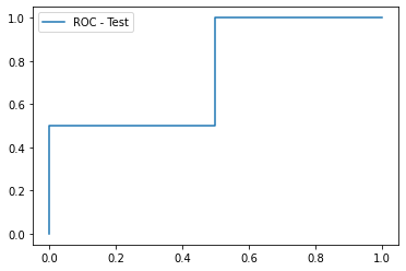
ここで、「あれ、思ってたものと違う」と感じる方がいるかもしれません。
それはその通りで、はじめに示したようなROC曲線を描くには、もっと多くのテストデータが必要です。
言い換えると、テストデータの数を増やせばよいということです。
今回は、4つしかないですからね。
また、今回はやっていませんが、ROC曲線の曲線を滑らかにカーブフィッティングすることもできます。
AUC
AUCは、Area Under Curveですから、ROC曲線下の面積のことを指します。
面積を求めれば良いので、この例では、簡単に求めることができます。
AUCが1に近いほどモデルの分類精度が良いことを意味します。
算出の方法は、先ほどのROC曲線を見ながら考えると考えやすいです。
グラフから、真陽性率が0.5であるバー(0.1きざみ)が5つと、真陽性率が1.0であるバーが5つあることが分かるので、単純な計算から0.75であることが分かります。
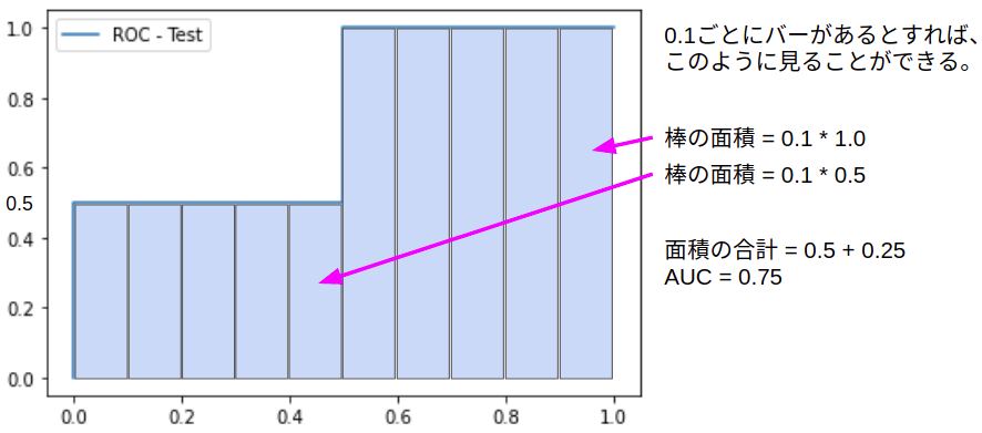
scikit-learnを用いても同じ結果になります。
# サンプルコード
import matplotlib.pyplot as plt
# しきい値[0.8 , 0.4 , 0.5 , 0.35 , 0.1]
tpr = [0, 0.5, 0.5, 0.5, 1.0 , 1.0]
fpr = [0, 0.0, 0.0, 0.5, 0.5 , 1.0]
# プロット
plt.plot(fpr, tpr, label="ROC - Test")
# 凡例の表示
plt.legend()
# プロット表示
plt.show()

# AUC
import numpy as np
from sklearn.metrics import roc_auc_score, auc

y = [0,0,1,1]
pred = [0.1, 0.4, 0.35, 0.8]
print(roc_auc_score(y,pred))
print(auc(fpr,tpr))

# 出力は省略しますが、0.75になります
ただし、ROC曲線がこだわりのある曲線で描かれている場合には、単純な棒グラフの長方形でだけでなく、台形も考えばければ無ければならなくなるので、曲線の描き方によって、AUCの算出方法は変わります。
FROC
ROC曲線が理解できたら、次はFROCです。
FROCの使いどころについて、書いてみます。
ここからの内容は、参考資料に記載の@fpgdubostさんのGitHubに公開されているデータとコードをお借りして書かせていただいています。
FROCはFree-response Receiver Operating Characteristicの略です。
直訳しても、前半はカタカナで、フリーレスポンス受信者動作特性などと呼ばれます。
ROCは、1画像につきラベルが1つに限定されていました。
なにかの画像をモデルに入力して、その画像がみかんであるかどうかを予測させ、その精度を測ることができました。
しかし、1枚の画像の中に複数の目的のものがある場合は、ROCでは評価が難しくなります。
このような、1枚の画像に目的のものが複数含まれている画像を対象とした「検出」モデルの精度を評価する手法がFROC解析です(応用は出来ますが、ここでは検出を対象としています)。
検出モデルは、二値分類モデルとは異なり、目的とするものの位置を予測するモデルです。
例えば、画像のなかに複数のみかんがあった場合、画像のどこにみかんがあるかを予測するモデルなどがそうです。
この中から、
ここにみかんがありますとモデルが検出できれば、そのモデルは精度が高いというわけです。
FROCは1枚の画像に目的のものが1個しかない、あるいは、含まれていない画像も対象にできます。
(故に、アンバランスデータを対象とした検出にロバスト性が高いと言われているようです。:自信がないのでカッコ)
FROCの解析では、ROCと同様に、左上にいくほど精度が高いと判断されるFROC曲線を描くことができます。
FROC曲線の縦軸は、ROC曲線と同じ真陽性率です。
一方、横軸はROC曲線とは違って、FPI:false positives per imagesで表わされます。
これは、1画像あたりの偽陽性数です。偽陽性率ではありません。
では、みかん検出モデルが、みかんを検出できるかテストしたいとしましょう。
上記の画像の場合、正解ラベル画像はこのように表されます。
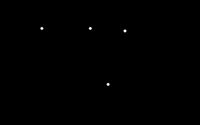
画像上にみかんが写っている場所がピクセル値が最大になっています。
点の大きさは任意ですが、一定です。
このような正解ラベル画像は、グラウンド・トゥルース画像とも呼ばれます。
そして、このテスト画像を検出モデルが予測した結果がこのようになったとします。

人が見れば、「ああ、モヤっとしているところが"りんご"だろう」と考えつくのですが、機械はそれが出来ないので、評価してあげる必要があるわけです。
理想的には、みかんの領域だけを機械が自動的に検出してくれるのがベストです。
理想が叶うと、真陽性率は100%、偽陽性の数は0個ということになります。
上述の図の例では、予測結果の斑点がみかん候補を意味しています。
このように、実際に予測させてみると、りんごをみかんと間違う(偽陽性)あるいはその反対(偽陰性)のケースが伴う場合があることがわかります。
このようにばらつく検出精度をFROCで評価したいということになります。
どうするかと言うと、
この予測画像内の斑点のコントラストは予測確率に比例しています。
この例では、予測確率が0.0の場合は画像上のピクセル値は0、予測確率1.0の場合はピクセル値は255です。
予測確率にしきい値を設ければ、ROC曲線を描いたときのように各しきい値での予測結果を得ることができます。
そして、それは画像として表現できます。
画像にしきい値を設定すると、「ある画素以上の領域をみかん候補としよう」と決めることができるというわけです。
例えば、しきい値を0, 63, 127, 191, 255の5段階に設定すれば、このような画像になります。
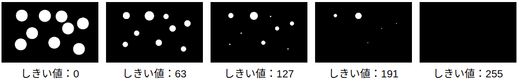
このようにしきい値を設けて画像を作れば、グラウンド・トゥルースと重なりあう斑点の数から真陽性率を、グラウンド・トゥルースと重なっていないが「みかん」と予測された斑点の数から偽陽性の数を求めることができます。
FROCもROCと同様に、このようにしきい値を変化させることでFROC曲線を描くためのプロット点を得られるというわけです。
では、pythonのライブラリをお借りして、実行してみたいと思います。
コードは、末尾に転載します。少し長いですが、そのままColabなどでまるごとコピペして使えます。
このように実行します。
import cv2
np.random.seed(1)
# parameters
save_path = 'FROC_example2.pdf' # 結果グラフの保存先
nbr_of_thresholds = 40 # しきい値の数
range_threshold = [0.1,.99] # しきい値の範囲。ピクセルは0-1に正規化されるので、この範囲で指定。
allowedDistance = 10 # グラウンド・トゥルースと離れたときの許容ピクセル数
# read the data
ground_truth = np.expand_dims(cv2.imread('ground_truth.png',cv2.IMREAD_GRAYSCALE),axis=0)
proba_map = np.expand_dims(cv2.imread('proba_map.png',cv2.IMREAD_GRAYSCALE),axis=0)
print(ground_truth.shape)
print(proba_map.shape)
ground_truth = np.float32(ground_truth)
proba_map = np.float32(proba_map)
# compute FROC
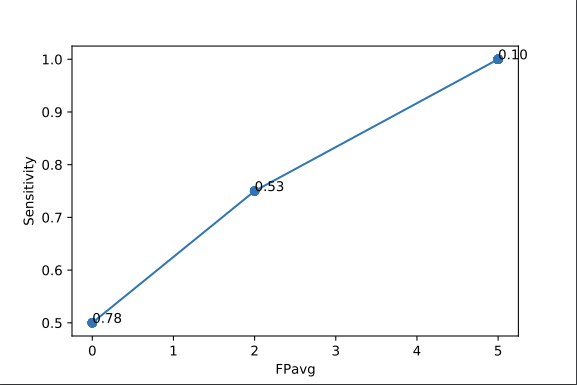
sensitivity_list, FPavg_list, threshold_list = computeFROC(proba_map,ground_truth, allowedDistance, nbr_of_thresholds, range_threshold)
# plot FROC
plotFROC(FPavg_list,sensitivity_list,save_path, threshold_list)
実行結果はこのようになります(図中の横軸がFPavg(偽陽性の数の平均)と表記されていますが、実際には1枚しか画像を使っていないので、平均ではありません)。
補足ですが、今回は一枚の画像の中の複数のみかんを対象として書いていますが、複数枚の画像セットの中の複数のみかんの検出精度を評価することもできます。
この場合は、しきい値ごとに、各画像で真陽性率を算出して、偽陽性数をカウントした後、全画像分のこれらの平均をそれぞれ求め、FROC曲線を描きます。
この理由で、このFROCコードで出力されるFROC曲線図の横軸ラベル名にはavgがついています。
画像一枚からFROCを行うときは、FPと表記したほうが適切です。
用途としては、例えば、医療の検査として実施されるCTスキャン画像などを用いる場合などが当てはまります。
Reference
- 参考にさせていただいたFROCのコード:https://github.com/fpgdubost/FROC
- 参考にさせていただいた文脈:https://www.clg.niigata-u.ac.jp/~medimg/practice_medical_imaging/roc/3lfroc/index.htm
- http://europepmc.org/backend/ptpmcrender.fcgi?accid=PMC2776072&blobtype=pdf
import matplotlib
matplotlib.use('Agg')
import matplotlib.pyplot as plt
import numpy as np
from scipy import ndimage
from scipy.spatial.distance import euclidean
from scipy.optimize import linear_sum_assignment
import pandas as pd
from pdb import set_trace as bp
import os

def computeAssignment(list_detections,list_gt,allowedDistance,save_disagreement=False):
    #the assignment is based on the hungarian algorithm
    #https://docs.scipy.org/doc/scipy-0.18.1/reference/generated/scipy.optimize.linear_sum_assignment.html
    #https://en.wikipedia.org/wiki/Hungarian_algorithm

    #build cost matrix
    #rows: GT
    #columns: detections
    cost_matrix = np.zeros([len(list_gt),len(list_detections)])
    for i, pointR1 in enumerate(list_gt):
        for j, pointR2 in enumerate(list_detections):
            cost_matrix[i,j] = euclidean(pointR1,pointR2)

    #perform assignment
    row_ind, col_ind = linear_sum_assignment(cost_matrix)

    #threshold points too far
    row_ind_thresholded = []
    col_ind_thresholded = []
    for i in range(len(row_ind)):
        if cost_matrix[row_ind[i],col_ind[i]] < allowedDistance:
            row_ind_thresholded.append(row_ind[i])
            col_ind_thresholded.append(col_ind[i])

    #save coord FP and FN
    if save_disagreement:
        #just copy the lists and remove correct detections
        list_FN = list(list_gt) #list() to copy
        list_FP = list(list_detections)
        for i in range(len(row_ind_thresholded)):
            list_FN.remove(list_gt[row_ind_thresholded[i]])
            list_FP.remove(list_detections[col_ind_thresholded[i]])

    #compute stats
    P = len(list_gt)
    TP = len(row_ind_thresholded)
    FP = len(list_detections) - TP

    if save_disagreement:
        return P,TP,FP,list_FP,list_FN
    else:
        return P,TP,FP


def computeFROCfromListsMatrix(list_ids,list_detections,list_gt,allowedDistance):
    #list_detection: first dimlension: number of images
    #list_gt: first dimlension: number of images

    #get maximum number of detection per image across the dataset
    max_nbr_detections = 0
    for detections in list_detections:
        if len(detections) > max_nbr_detections:
            max_nbr_detections = len(detections)

    sensitivity_matrix = pd.DataFrame(columns=list_ids)
    FP_matrix = pd.DataFrame(columns=list_ids)

    #iterate over 'thresholds'
    for i in range(1,max_nbr_detections):
        sensitivity_per_image = {}
        FP_per_image = {}
        #iterate over scans
        for image_nbr, gt in enumerate(list_gt):
            image_id = list_ids[image_nbr]
            if len(gt) > 0:  #check that ground truth contains at least one annotation
                if i <= len(list_detections[image_nbr]): #if there are detections
                    #compute P, TP, FP per image
                    detections = list_detections[image_nbr][-i]
                    P,TP,FP = computeAssignment(detections,gt,allowedDistance)
                else:
                    P = len(gt)
                    TP,FP = 0,0

                #append results to list
                FP_per_image[image_id] = FP
                sensitivity_per_image[image_id] = TP*1./P

            elif len(gt) == 0 and i <= len(list_detections[image_nbr]): #if no annotations but detections
                FP = len(list_detections[image_nbr][-i])
                FP_per_image[image_id] = FP
                sensitivity_per_image[image_id] = None

        sensitivity_matrix = sensitivity_matrix.append(sensitivity_per_image,ignore_index=True)
        FP_matrix = FP_matrix.append(FP_per_image,ignore_index=True)

    return sensitivity_matrix.transpose(), FP_matrix.transpose()

def computeFROCfromLists(list_detections,list_gt,allowedDistance):
    #get maximum number of detection per image across the dataset
    max_nbr_detections = 0
    for detections in list_detections:
        if len(detections) > max_nbr_detections:
            max_nbr_detections = len(detections)

    sensitivity_list = []
    FPavg_list = []
    sensitivity_list_std = []
    FPavg_list_std = []

    for i in range(max_nbr_detections):
        sensitivity_list_per_image = []
        FP_list_per_image = []
        for image_nbr, gt in enumerate(list_gt):
            if len(gt) > 0:  #check that ground truth contains at least one annotation
                if i <= len(list_detections[image_nbr]): #if there are detections
                    #compute P, TP, FP per image
                    detections = list_detections[image_nbr][-i]
                    P,TP,FP = computeAssignment(detections,gt,allowedDistance)
                else:
                    P = len(gt)
                    TP,FP = 0,0

                #append results to list
                FP_list_per_image.append(FP)
                sensitivity_list_per_image.append(TP*1./P)

            elif len(gt) == 0 and i <= len(list_detections[image_nbr]): #if no annotations but detections
                FP = len(list_detections[image_nbr][-i])
                FP_list_per_image.append(FP)
                sensitivity_list_per_image.append(None)

        #average sensitivity and FP over the proba map, for a given threshold
        sensitivity_list.append(np.mean(sensitivity_list_per_image))
        FPavg_list.append(np.mean(FP_list_per_image))
        sensitivity_list_std.append(np.std(sensitivity_list_per_image))
        FPavg_list_std.append(np.std(FP_list_per_image))

    return sensitivity_list, FPavg_list, sensitivity_list_std, FPavg_list_std

def computeConfMatElements(thresholded_proba_map, ground_truth, allowedDistance):

    if allowedDistance == 0 and type(ground_truth) == np.ndarray:
        P = np.count_nonzero(ground_truth)
        TP = np.count_nonzero(thresholded_proba_map*ground_truth)
        FP = np.count_nonzero(thresholded_proba_map - (thresholded_proba_map*ground_truth))
    else:

        #reformat ground truth to a list
        if type(ground_truth) == np.ndarray:
            #convert ground truth binary map to list of coordinates
            labels, num_features = ndimage.label(ground_truth)
            list_gt = ndimage.measurements.center_of_mass(ground_truth, labels, range(1,num_features+1))
        elif type(ground_truth) == list:
            list_gt = ground_truth
        else:
            raise ValueError('ground_truth should be either of type list or ndarray and is of type ' + str(type(ground_truth)))

        #reformat thresholded_proba_map to a list
        labels, num_features = ndimage.label(thresholded_proba_map)
        list_proba_map = ndimage.measurements.center_of_mass(thresholded_proba_map, labels, range(1,num_features+1))

        #compute P, TP and FP
        P,TP,FP = computeAssignment(list_proba_map,list_gt,allowedDistance)

    return P,TP,FP

def computeFROC(proba_map, ground_truth, allowedDistance, nbr_of_thresholds=40, range_threshold=None):
    #INPUTS
    #proba_map : numpy array of dimension [number of image, xdim, ydim,...], values preferably in [0,1]
    #ground_truth: numpy array of dimension [number of image, xdim, ydim,...], values in {0,1}; or list of coordinates
    #allowedDistance: Integer. euclidian distance distance in pixels to consider a detection as valid (anisotropy not considered in the implementation)
    #nbr_of_thresholds: Interger. number of thresholds to compute to plot the FROC
    #range_threshold: list of 2 floats. Begining and end of the range of thresholds with which to plot the FROC
    #OUTPUTS
    #sensitivity_list_treshold: list of average sensitivy over the set of images for increasing thresholds
    #FPavg_list_treshold: list of average FP over the set of images for increasing thresholds
    #threshold_list: list of thresholds

    #rescale ground truth and proba map between 0 and 1
    proba_map = proba_map.astype(np.float32)
    proba_map = (proba_map - np.min(proba_map)) / (np.max(proba_map) - np.min(proba_map))
    if type(ground_truth) == np.ndarray:
        #verify that proba_map and ground_truth have the same shape
        if proba_map.shape != ground_truth.shape:
            raise ValueError('Error. Proba map and ground truth have different shapes.')

        ground_truth = ground_truth.astype(np.float32)
        ground_truth = (ground_truth - np.min(ground_truth)) / (np.max(ground_truth) - np.min(ground_truth))

    #define the thresholds
    if range_threshold == None:
        threshold_list = (np.linspace(np.min(proba_map),np.max(proba_map),nbr_of_thresholds)).tolist()
    else:
        threshold_list = (np.linspace(range_threshold[0],range_threshold[1],nbr_of_thresholds)).tolist()

    sensitivity_list_treshold = []
    FPavg_list_treshold = []
    #loop over thresholds
    for threshold in threshold_list:
        sensitivity_list_proba_map = []
        FP_list_proba_map = []
        #loop over proba map
        for i in range(len(proba_map)):

            #threshold the proba map
            thresholded_proba_map = np.zeros(np.shape(proba_map[i]))
            thresholded_proba_map[proba_map[i] >= threshold] = 1

            #save proba maps
#            imageio.imwrite('thresholded_proba_map_'+str(threshold)+'.png', thresholded_proba_map)

            #compute P, TP, and FP for this threshold and this proba map
            P,TP,FP = computeConfMatElements(thresholded_proba_map, ground_truth[i], allowedDistance)

            #append results to list
            FP_list_proba_map.append(FP)
            #check that ground truth contains at least one positive
            if (type(ground_truth) == np.ndarray and len(np.nonzero(ground_truth)) > 0) or (type(ground_truth) == list and (len(ground_truth) > 0)):
              sensitivity_list_proba_map.append(TP*1./P)


        #average sensitivity and FP over the proba map, for a given threshold
        sensitivity_list_treshold.append(np.mean(sensitivity_list_proba_map))
        FPavg_list_treshold.append(np.mean(FP_list_proba_map))

    return sensitivity_list_treshold, FPavg_list_treshold, threshold_list

def plotFROC(x,y,save_path,threshold_list=None):
    plt.figure()
    plt.plot(x,y, 'o-')
    plt.xlabel('FPavg')
    plt.ylabel('Sensitivity')

    #annotate thresholds
    if threshold_list != None:
        #round thresholds
        threshold_list = [ '%.2f' % elem for elem in threshold_list ]
        xy_buffer = None
        for i, xy in enumerate(zip(x, y)):
            if xy != xy_buffer:
                plt.annotate(str(threshold_list[i]), xy=xy, textcoords='data')
                xy_buffer = xy

    plt.savefig(save_path)
    #plt.show()