14杯目セキュリティうどん（かまたま）勉強会

14杯目セキュリティうどん（かまたま）勉強会のまとめ

000 はじめに

「Python入門と機械学習によるマルウェア検知」というタイトルでトレンドマイクロのエンジニア
トレンドマイクロ株式会社 上級スレットディフェンスエキスパート 新井 悠 氏によるハンズオン形式のワークショップが開催されました。

14杯目セキュリティうどん（かまたま）勉強会
http://sec-udon.jpn.org/doku.php?id=workshop:14th

001 自己紹介

定員50名（満員御礼）の参加者がそれぞれ自己紹介をしました。開催地香川の他、
千葉、熊本、島根、愛媛、徳島など全国各地から集まりました。
職種もさまざまですが、セキュリティ関連業務の方や、官公庁の方もいらっしゃいました。

010 Python入門

何はともあれ Python入門 です。Python3 をインストールし、Anaconda も入れます。
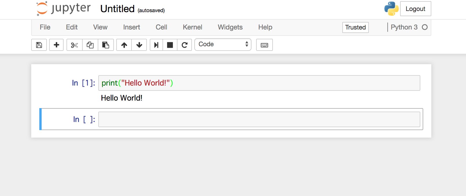
jupyter notebook で説明されます。

> jupyter notebook

コマンドで実行し、何はともあれ "Hello World!" ですね。はい、入門終了。

011 マルウェア解析

次にマルウェアを解析するのですが、ここで、pefile というライブラリが必要になりますので、以下のようにしてインストールします。

> pip install pefile

その後、以下のようにすると、exe のヘッダが丸見えです。

# coding: utf-8
import pefile

# ファイルパスは各自
PATH=u'/Users/taniokah/Projects/udon/data/PE-samples/TestApp.exe'
pe = pefile.PE(PATH)
print("{0}".format(pe.FILE_HEADER))

[IMAGE_FILE_HEADER]
0xE4       0x0   Machine:                       0x14C     
0xE6       0x2   NumberOfSections:              0x7       
0xE8       0x4   TimeDateStamp:                 0x59194A4D [Mon May 15 06:27:25 2017 UTC]
0xEC       0x8   PointerToSymbolTable:          0x0       
0xF0       0xC   NumberOfSymbols:               0x0       
0xF4       0x10  SizeOfOptionalHeader:          0xE0      
0xF6       0x12  Characteristics:               0x102     

print("{0}".format(pe.DOS_HEADER))

[IMAGE_DOS_HEADER]
0x0        0x0   e_magic:                       0x5A4D    
0x2        0x2   e_cblp:                        0x90      
0x4        0x4   e_cp:                          0x3       
0x6        0x6   e_crlc:                        0x0       
0x8        0x8   e_cparhdr:                     0x4       
0xA        0xA   e_minalloc:                    0x0       
0xC        0xC   e_maxalloc:                    0xFFFF    
0xE        0xE   e_ss:                          0x0       
0x10       0x10  e_sp:                          0xB8      
0x12       0x12  e_csum:                        0x0       
0x14       0x14  e_ip:                          0x0       
0x16       0x16  e_cs:                          0x0       
0x18       0x18  e_lfarlc:                      0x40      
0x1A       0x1A  e_ovno:                        0x0       
0x1C       0x1C  e_res:                         
0x24       0x24  e_oemid:                       0x0       
0x26       0x26  e_oeminfo:                     0x0       
0x28       0x28  e_res2:                        
0x3C       0x3C  e_lfanew:                      0xE0      

# IMAGE_FILE_EXECUTABLE_IMAGE 0x0002
if pe.FILE_HEADER.Characteristics & 0x0002:
    print("IMAGE_FILE_EXECUTABLE_IMAGE")
#IMAGE_FILE_32BIT_MACHINE 0x0100
if pe.FILE_HEADER.Characteristics & 0x0100:
    print("IMAGE_FILE_32BIT_MACHINE")

IMAGE_FILE_EXECUTABLE_IMAGE
IMAGE_FILE_32BIT_MACHINE

print("{0}".format(pe.OPTIONAL_HEADER))

[IMAGE_OPTIONAL_HEADER]
0xF8       0x0   Magic:                         0x10B     
0xFA       0x2   MajorLinkerVersion:            0xB       
0xFB       0x3   MinorLinkerVersion:            0x0       
0xFC       0x4   SizeOfCode:                    0x4400    
0x100      0x8   SizeOfInitializedData:         0x4000    
0x104      0xC   SizeOfUninitializedData:       0x0       
0x108      0x10  AddressOfEntryPoint:           0x11131   
0x10C      0x14  BaseOfCode:                    0x1000    
0x110      0x18  BaseOfData:                    0x1000    
0x114      0x1C  ImageBase:                     0x400000  
0x118      0x20  SectionAlignment:              0x1000    
0x11C      0x24  FileAlignment:                 0x200     
0x120      0x28  MajorOperatingSystemVersion:   0x6       
0x122      0x2A  MinorOperatingSystemVersion:   0x0       
0x124      0x2C  MajorImageVersion:             0x0       
0x126      0x2E  MinorImageVersion:             0x0       
0x128      0x30  MajorSubsystemVersion:         0x6       
0x12A      0x32  MinorSubsystemVersion:         0x0       
0x12C      0x34  Reserved1:                     0x0       
0x130      0x38  SizeOfImage:                   0x1D000   
0x134      0x3C  SizeOfHeaders:                 0x400     
0x138      0x40  CheckSum:                      0x0       
0x13C      0x44  Subsystem:                     0x3       
0x13E      0x46  DllCharacteristics:            0x8140    
0x140      0x48  SizeOfStackReserve:            0x100000  
0x144      0x4C  SizeOfStackCommit:             0x1000    
0x148      0x50  SizeOfHeapReserve:             0x100000  
0x14C      0x54  SizeOfHeapCommit:              0x1000    
0x150      0x58  LoaderFlags:                   0x0       
0x154      0x5C  NumberOfRvaAndSizes:           0x10      

100 主成分分析

機械学習は、データ駆動の手法です。pandasとnumpyでデータを読み込んで加工しましょう。

import glob
import pandas as pd

df = pd.DataFrame(columns=["malware","VirtualAddress","ResourceSize","DebugSize","IATSize"])

# 特徴抽出対象ファイルの列挙
PATH = u'/Users/taniokah/Projects/udon/data/PE-samples/*'
files = glob.glob(PATH)

# PEで特徴量の抽出 pefile.DIRECTORY_ENTRY['IMAGE_DIRECTORY_ENTRY_IMPORT']
for file in files:
    data = pefile.PE(file)
    VA = data.OPTIONAL_HEADER.DATA_DIRECTORY[1].VirtualAddress
    RS = data.OPTIONAL_HEADER.DATA_DIRECTORY[2].Size
    DS = data.OPTIONAL_HEADER.DATA_DIRECTORY[6].Size
    IATSize = data.OPTIONAL_HEADER.DATA_DIRECTORY[1].Size
    newdf = pd.DataFrame([[0, VA, RS, DS, IATSize]], columns=["malware", "VirtualAddress", "ResourceSize", "DebugSize", "IATSize"])

    df = df.append(newdf, ignore_index=True)

df

	malware	VirtualAddress	ResourceSize	DebugSize	IATSize
0	0	106496	1084	56	60
1	0	102400	1084	56	60
2	0	106496	1084	56	80
3	0	102400	1084	56	80
4	0	106496	1084	56	80

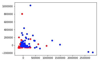
さらに、主成分分析(PCA)を使ってテストデータを可視化します。

import pandas as pd
import numpy as np
import matplotlib.pyplot as plt
from sklearn.decomposition import PCA

PATH= '/Users/taniokah/Projects/udon/data/'

df1 = pd.read_csv(PATH+'malware.csv')
df2 = pd.read_csv(PATH+'benign.csv')

X_reduced = PCA(n_components=2).fit_transform(np.array(df1)[:,2:])
Y_reduced = PCA(n_components=2).fit_transform(np.array(df2)[:,2:])

plt.scatter(X_reduced[:,0], X_reduced[:,1], c="red")
plt.scatter(Y_reduced[:,0], Y_reduced[:,1], c="blue")
plt.show()

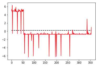
101 線形分離

線形分離（LDA）で2次元データを1次元に次元縮約してみます。

from sklearn.discriminant_analysis import LinearDiscriminantAnalysis as LDA

df = pd.read_csv(PATH+'union.csv')

X_reduced = LDA(n_components=1).fit_transform(np.array(df)[:,2:], np.array(df)[:,1])

plt.plot(X_reduced[:,0], c="red")
plt.hlines(y=0.2, xmin=0, xmax=355, linestyle="dashed")
plt.show()

/Users/taniokah/.pyenv/versions/anaconda3-5.0.1/lib/python3.6/site-packages/sklearn/discriminant_analysis.py:388: UserWarning: Variables are collinear.
  warnings.warn("Variables are collinear.")

110 k近傍法

いよいよ、本格的に機械学習によるマルウェアの識別をします。ここでは、k近傍法(kNN)を使います。

from sklearn.neighbors import KNeighborsClassifier

df = pd.read_csv(PATH+'union.csv')
clf_k = KNeighborsClassifier(n_neighbors=3)
clf_k.fit(np.array(df)[:,2:], np.array(df)[:,1])

test_df = pd.read_csv(PATH+'test2.csv')
output = clf_k.predict(np.array(test_df)[:,2:])

for i in output:
    if i == 0:
        print("not malware")
    elif i == 1: 
        print("malware")

malware
not malware
malware
malware
not malware
not malware
malware
not malware
not malware
not malware
not malware
not malware
not malware
not malware
malware
not malware
not malware
not malware
not malware
not malware
not malware
malware
not malware
not malware
not malware

学習用のデータを読み込んで、テスト用で判定してみます。
結果は、malwere と not malware と分類できました。どの程度の精度が出ているか見てみます。

from sklearn.metrics import accuracy_score
accuracy_score(np.array(test_df)[:,1], output)

0.56000000000000005

df = pd.read_csv(PATH+'union.csv')
test_df = pd.read_csv(PATH+'test2.csv')

for i in range(1, 20):
    clf_k = KNeighborsClassifier(n_neighbors=i)
    clf_k.fit(np.array(df)[:,2:], np.array(df)[:,1])
    output = clf_k.predict(np.array(test_df)[:,2:])
    print("n_neighbors={0} {1}".format(i, accuracy_score(np.array(test_df)[:,1], output)))

n_neighbors=1 0.32
n_neighbors=2 0.4
n_neighbors=3 0.56
n_neighbors=4 0.52
n_neighbors=5 0.52
n_neighbors=6 0.52
n_neighbors=7 0.52
n_neighbors=8 0.52
n_neighbors=9 0.52
n_neighbors=10 0.52
n_neighbors=11 0.52
n_neighbors=12 0.52
n_neighbors=13 0.76
n_neighbors=14 0.76
n_neighbors=15 0.76
n_neighbors=16 0.76
n_neighbors=17 0.76
n_neighbors=18 0.76
n_neighbors=19 0.76

for i in range(1, 30):
    clf_k = KNeighborsClassifier(n_neighbors=i)
    clf_k.fit(np.array(df)[:,2:], np.array(df)[:,1])
    output = clf_k.predict(np.array(test_df)[:,2:])
    print("n_neighbors={0} {1}".format(i, accuracy_score(np.array(test_df)[:,1], output)))

n_neighbors=1 0.32
n_neighbors=2 0.4
n_neighbors=3 0.56
n_neighbors=4 0.52
n_neighbors=5 0.52
n_neighbors=6 0.52
n_neighbors=7 0.52
n_neighbors=8 0.52
n_neighbors=9 0.52
n_neighbors=10 0.52
n_neighbors=11 0.52
n_neighbors=12 0.52
n_neighbors=13 0.76
n_neighbors=14 0.76
n_neighbors=15 0.76
n_neighbors=16 0.76
n_neighbors=17 0.76
n_neighbors=18 0.76
n_neighbors=19 0.76
n_neighbors=20 0.72
n_neighbors=21 0.68
n_neighbors=22 0.68
n_neighbors=23 0.6
n_neighbors=24 0.6
n_neighbors=25 0.6
n_neighbors=26 0.56
n_neighbors=27 0.6
n_neighbors=28 0.4
n_neighbors=29 0.36

111 まとめ

Pythonや機械学習初心者が多かったようなので、ちょうどよい内容かな？と思った。
個人的には、もうちょっと機械学習に踏み込んで欲しかったです。

時間があまったので、LDAでも予測してみた。

from sklearn.discriminant_analysis import LinearDiscriminantAnalysis as LDA

df = pd.read_csv(PATH+'union.csv')
test_df = pd.read_csv(PATH+'test2.csv')

clf = LDA()
clf.fit(np.array(df)[:,2:], np.array(df)[:,1])
output = clf.predict(np.array(test_df)[:,2:])
print("lda accuracy = {0}".format(accuracy_score(np.array(test_df)[:,1], output)))

lda accuracy = 0.64

64%ということで、kNNより悪い。残念。SVMやNB、DNNを使えばもっとあげられるかな？