下式で定義される関数$f(\textbf{x})$を用いて、入力ベクトル$\textbf{x}=(x_1, x_2, \cdots , x_N)$の2値分類を行うことを考える。
f(\textbf{x}) = \phi(\sum_{p=1}^{P} \sum_{n=1}^{N} w_{n,p} \, {x_n} ^p + w_{0})\\

\\

 \phi(y) =

  \left\{
    \begin{array}{l}
      1 \quad (y \geq 0) \\
      -1 \quad (otherwise)
    \end{array}
  \right.
ここで、$w_{n,p}$は重みパラメータ、$N$は入力ベクトル$\textbf{x}$の次元、$P$は多項式の次数である。重みパラメータ$w_{n,p}$は平均2乗誤差
l(\textbf{W}) = \sum_{i=1}^{I} (y_i - f(\textbf{x}_i))^2
を確率的勾配降下法により最小化することにより得られる。学習時の重みパラメータ$w_{n,p}$更新式の一例を下記に示す。
 w_{0} \leftarrow w_{0} + \eta \sum_{i=1}^{I} (y_i - f(\textbf{x}_i)) \\
 w_{n,p} \leftarrow w_{n,p} + \eta \sum_{i=1}^{I} ((y_i - f(\textbf{x}_i)) ( \sum_{n=1}^{N} {x_{n,i}} \, ^{p} ))
$\eta$は学習率、$(\textbf{x}_i, y_i)$は$i$番目の教師データ、$I$はバッチサイズを表している。
$P=1$の時、関数$f(\textbf{x})$はよく知られている単純パーセプトロンに一致し、関数$\phi$に入力されるのは$\textbf{x}$の線形関数となる。一方、$P>1$の時には、関数$\phi$に入力されるのは$\textbf{x}$の多項式であり、線形関数ではなくなる。次数$P$を高くすることで、関数$f(\textbf{x})$の非線形性を強くすることができる。関数$f(\textbf{x})$は単純パーセプトロンを非線形化したものと考えられる。
次数$P$の影響をみるために、Irisのデータセットを用いて学習を行い、分類結果を可視化してみた。実験結果を下記に示す。
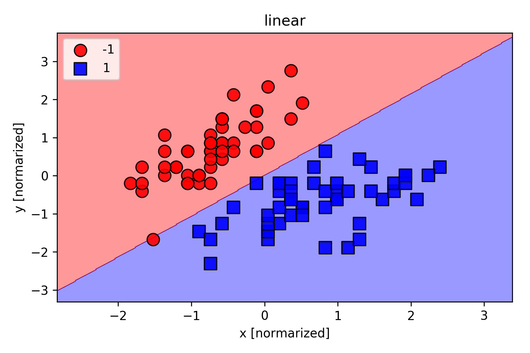
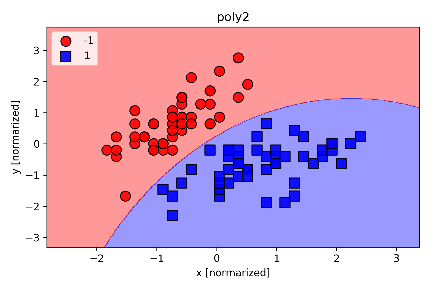
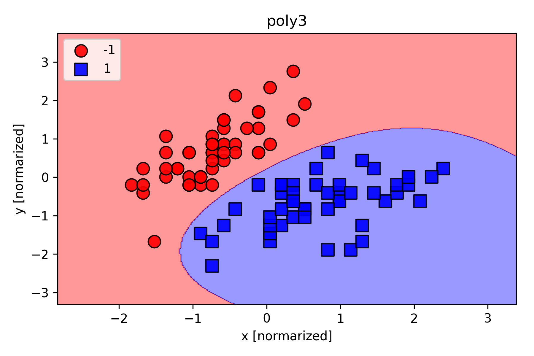
linearと書いてあるのが次数$P=1$の時の結果(単純パーセプトロン)で、poly2, poly3と書いてあるのが次数$P=2$, $P=3$の時の結果。次数$P$を高くすることで、複雑な分類にも対応できるようになることが分かる。
下記は実験に使用したソースコード。
MyClass.py
import numpy as np
from numpy.random import *


class MyClass(object):

    def __init__(self, eta=0.01, n_iter=10, shuffle=True, random_state=None, model='linear'):
        self.eta = eta
        self.n_iter = n_iter
        self.w_initialized = False
        self.shuffle = shuffle
        self.model=model
        if random_state:
            seed(random_state)

    def fit(self, X, y):
        self._initialize_weights(X.shape[1])
        self.cost_ = []
        for i in range(self.n_iter):
            if self.shuffle:
                X, y = self._shuffle(X, y)
            cost = []
            for xi, target in zip(X, y):
                cost.append(self._update_weights(xi, target))
            avg_cost = sum(cost) / len(y)
            self.cost_.append(avg_cost)
        return self

    def _shuffle(self, X, y):
        r = np.random.permutation(len(y))
        return X[r], y[r]

    def _initialize_weights(self, m):
        self.w1 = randn(m)
        self.w2 = randn(m)
        self.w3 = randn(m)
        self.b = randn(1)
        self.w_initialized = True

    def _update_weights(self, xi, target):
        output = self.activation(xi)
        error = (target - output)
        if self.model == 'linear':
            self.w1 += self.eta * xi * error
        elif self.model == 'poly2':
            self.w1 += self.eta * xi * error
            self.w2 += self.eta * (xi**2) * error
        elif self.model == 'poly3':
            self.w1 += self.eta * xi * error
            self.w2 += self.eta * (xi**2) * error
            self.w3 += self.eta * (xi**3) * error
        self.b += self.eta * error
        cost = 0.5 * error**2
        return cost

    def activation(self, X):
        if self.model == 'linear':
            return np.dot(X, self.w1) + self.b
        elif self.model == 'poly2':
            return np.dot(X, self.w1) + np.dot((X**2), self.w2) + self.b
        elif self.model == 'poly3':
            return np.dot(X, self.w1) + np.dot((X**2), self.w2) + np.dot((X**3), self.w3)  + self.b

    def predict(self, X):
        return np.where(self.activation(X) >= 0.0, 1, -1)
plot_decision_regions.py
import numpy as np
import matplotlib.pyplot as plt


def plot_decision_regions(X, y, classifier, resolution=0.02):

    '''
    https://github.com/rasbt/python-machine-learning-book/tree/master/code/ch02
    '''

    # setup marker generator and color map
    markers = ('o', 's', 'x', '^', 'v')
    colors = ('red', 'blue', 'lightgreen', 'gray', 'cyan')
    cmap = ListedColormap(colors[:len(np.unique(y))])

    # plot the decision surface
    x1_min, x1_max = X[:, 0].min() - 1, X[:, 0].max() + 1
    x2_min, x2_max = X[:, 1].min() - 1, X[:, 1].max() + 1
    xx1, xx2 = np.meshgrid(np.arange(x1_min, x1_max, resolution),
                           np.arange(x2_min, x2_max, resolution))
    Z = classifier.predict(np.array([xx1.ravel(), xx2.ravel()]).T)
    Z = Z.reshape(xx1.shape)
    plt.contourf(xx1, xx2, Z, alpha=0.4, cmap=cmap)
    plt.xlim(xx1.min(), xx1.max())
    plt.ylim(xx2.min(), xx2.max())

    # plot class samples
    for idx, cl in enumerate(np.unique(y)):
        plt.scatter(x=X[y == cl, 0], y=X[y == cl, 1],
                    alpha=0.9, c=cmap(idx), s=100,
                    edgecolor='black',
                    marker=markers[idx],
                    label=cl)
main.py
import matplotlib.pyplot as plt
import numpy as np
import pandas as pd
from numpy.random import *
from MyClass import MyClass
from plot_decision_regions import plot_decision_regions


# load dataset
df = pd.read_csv('https://archive.ics.uci.edu/ml/'
                 'machine-learning-databases/iris/iris.data', header=None)
df.tail()

# select setosa and versicolor
y = df.iloc[0:100, 4].values
y = np.where(y == 'Iris-setosa', -1, 1)

# extract x and y
X = df.iloc[0:100, [0,1]].values

# normarize X
X_std = np.copy(X)
X_std[:, 0] = (X[:, 0] - X[:, 0].mean()) / X[:, 0].std()
X_std[:, 1] = (X[:, 1] - X[:, 1].mean()) / X[:, 1].std()

model_names = ['linear', 'poly2', 'poly3']
for model in model_names:

    # import model
    ada = MyClass(n_iter=50, eta=0.01, random_state=1, model=model)

    # fitting
    ada.fit(X_std, y)

    # predict & plot
    plot_decision_regions(X_std, y, classifier=ada)
    plt.title(model)
    plt.xlabel('x [normarized]')
    plt.ylabel('y [normarized]')
    plt.legend(loc='upper left')
    plt.tight_layout()
    plt.savefig(model + '.png', dpi=300)
    plt.show()

    del ada
参考:
どやっ!