LSTMの誤差逆伝播

はじめに

ベクトルや行列を含む微分について の記事の続きで、LSTM の誤差逆伝播について取り上げます。

これも、書籍『詳解ディープラーニング』で LSTM の解説を読んだのが発端で、書籍中の誤差逆伝播の式が間違っていて、しかも簡単な間違いでもなく、かなり悩んだので、正しく扱ったらどうなるかを書いてみました。ポイントとしては多変数関数の微分の扱いになります。

なお、LSTM については他のページに包括的に書かれており、誤差逆伝播についても正確に書かれているので、全体的にはそちらを参考にしてください。この記事では誤差逆伝播の計算に焦点を絞って書きます。

モデルの定義

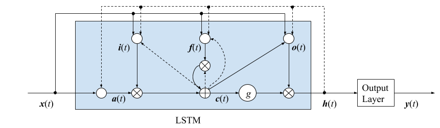
LSTM のブロック図は上のようになります。図中の点線は過去の信号を使うことを示しています。中に何も書いていない白丸は非線形活性化の処理を表しています。

以下、要素を表す添字のない小文字の変数はすべてベクトル、大文字の係数は行列とします。

• 入力 $x(t)$ と1つ前の時刻の隠れ層 $h(t-1)$ から $a(t)$ を作る。
  $$a(t)=f(\hat a(t))=f(W_\mathrm ax(t)+U_\mathrm ah(t-1)+b_\mathrm a)$$

• $a(t)$ と自己の1つ前の時刻の値 $c(t-1)$ にそれぞれ入力ゲート、忘却ゲートを掛けて足したものを CEC（メモリセル） とする。
  $$c(t)=i(t)\odot a(t)+f(t)\odot c(t-1)$$

• $c(t)$ を活性化して、出力ゲートを掛けたものを隠れ層の出力とする。
  $$h(t)=o(t)\odot g(c(t))$$

• 入力ゲート $i(t)$、忘却ゲート $f(t)$¹、出力ゲート $o(t)$ は以下のように作る。²

$$
i(t)=\sigma(\hat i(t))=\sigma(W_\mathrm ix(t)+U_\mathrm ih(t-1)+v_\mathrm i\odot c(t-1)+b_\mathrm i)$$

$$f(t)=\sigma(\hat f(t))=\sigma(W_\mathrm fx(t)+U_\mathrm fh(t-1)+v_\mathrm f\odot c(t-1)+b_\mathrm f)$$

$$o(t)=\sigma(\hat o(t))=\sigma(W_\mathrm ox(t)+U_\mathrm oh(t-1)+v_\mathrm o\odot c(t)+b_\mathrm o)$$

• 隠れ層 $h(t)$ から出力層 $y(t)$ を作る。³
  $$y(t)=Vh(t)+c$$

誤差関数の微分

$W_{\mathrm{i,f,o,a}}$, $U_{\mathrm{i,f,o,a}}$, $v_{\mathrm{i,f,o}}$, $b_{\mathrm{i,f,o,a}}$, $V$, $c$ が重み係数であり、誤差関数 $E$ をこれらについて微分する必要があります。

通常のニューラルネットワークと同様、重み係数で微分した結果は、入力信号と誤差逆伝播で得られる誤差信号のテンソル積になります。ただし、活性化関数があれば、活性化関数の微係数も掛けます。例えば、$\partial E/\partial W_\mathrm i$ は
$$
\frac{\partial E}{\partial W_\mathrm i} = \sum_t e_\mathrm i(t)\odot \sigma'(\hat i(t))x(t)^T
$$

であり⁴、他の重み係数についても同様の形になります。

このように、誤差関数を重み係数で微分すると、誤差信号 $e_{\mathrm{i,f,o,a}}(t)$ が出てくるので、これらを誤差逆伝播計算で求める必要があります。

誤差逆伝播

$e_{\mathrm{i,f,o,a}}(t)$ を求めるため、$i(t)$, $f(t)$, $o(t)$, $a(t)$ の1つ先の伝播先を見ます。関連するモデル式は以下の2つです。

\begin{aligned}
c(t)&=i(t)\odot a(t)+f(t)\odot c(t-1) \\
h(t)&=o(t)\odot g(c(t))
\end{aligned}

したがって、各信号の伝播先は以下の通りです。
$$
i(t)\rightarrow c(t), \ f(t)\rightarrow c(t), \ o(t)\rightarrow h(t), \ a(t)\rightarrow c(t)
$$

これらの誤差信号を $e_\mathrm c(t), e_\mathrm h(t)$ とおくと、$e_{\mathrm{i,f,o,a}}(t)$ は

\begin{aligned}
e_\mathrm i(t)&= \frac{\partial c(t)}{\partial i(t)} \frac{\partial E}{\partial c(t)} = a(t) \odot e_\mathrm c(t) \\
e_\mathrm f(t)&=\frac{\partial c(t)}{\partial f(t)} \frac{\partial E}{\partial c(t)} = c(t-1) \odot e_\mathrm c(t) \\
e_\mathrm o(t)&=\frac{\partial h(t)}{\partial o(t)} \frac{\partial E}{\partial h(t)} = g(c(t)) \odot e_\mathrm h(t) \\
e_\mathrm a(t)&=\frac{\partial c(t)}{\partial a(t)} \frac{\partial E}{\partial c(t)} = i(t) \odot e_\mathrm c(t)
\end{aligned}

となり、すべて $e_\mathrm c(t)$, $e_\mathrm h(t)$ で表されることが分かります。よって、$e_\mathrm c(t)$, $e_\mathrm h(t)$ を計算できれば良いことになります。

ここまでは、書籍に書かれている通りですが、この後に大きな間違いがあります。$c(t), h(t)$ は複数の信号に伝播しており、これらの複数の信号はすべて誤差関数に寄与しています。したがって、$e_\mathrm c(t)$, $e_\mathrm h(t)$ を計算するには、$c(t)$, $h(t)$ が伝播する先の信号をすべて書き出す必要があります。

$c(t)$ について伝播先を実際に書き出してみます。関連するモデル式は以下の5つです。

\begin{aligned}
h(t)&=o(t)\odot g(c(t)) \\
c(t)&=i(t)\odot a(t)+f(t)\odot c(t-1) \\
i(t)&=\sigma(\hat i(t))=\sigma(W_\mathrm ix(t)+U_\mathrm ih(t-1)+v_\mathrm i\odot c(t-1)+b_\mathrm i)\\
f(t)&=\sigma(\hat f(t))=\sigma(W_\mathrm fx(t)+U_\mathrm fh(t-1)+v_\mathrm f\odot c(t-1)+b_\mathrm f)\\
o(t)&=\sigma(\hat o(t))=\sigma(W_\mathrm ox(t)+U_\mathrm oh(t-1)+v_\mathrm o\odot c(t)+b_\mathrm o)
\end{aligned}

したがって、$c(t)$ の伝播先は以下のようになります。
$$
c(t)\rightarrow h(t),\ c(t+1),\ i(t+1),\ f(t+1),\ o(t)
$$

$e_\mathrm c(t)$ はこれらのすべての信号からの誤差逆伝播の和になります。

\begin{aligned}
e_\mathrm c(t)= & \ \frac{\partial h(t)}{\partial c(t)} \frac{\partial E}{\partial h(t)} + 
\frac{\partial c(t+1)}{\partial c(t)} \frac{\partial E}{\partial c(t+1)} \\
& + \frac{\partial i(t+1)}{\partial c(t)} \frac{\partial E}{\partial i(t+1)} +
\frac{\partial f(t+1)}{\partial c(t)} \frac{\partial E}{\partial f(t+1)} + 
\frac{\partial o(t)}{\partial c(t)} \frac{\partial E}{\partial o(t)} \\
= & \ o(t)\odot g'(c(t))\odot e_\mathrm h(t) + 
f(t+1) \odot e_\mathrm c(t+1) \\
& + v_\mathrm i \odot e_\mathrm i(t+1) +
v_\mathrm f \odot e_\mathrm f(t+1) + v_\mathrm o \odot e_\mathrm o(t)
\end{aligned}

5つの項のうち、$e_\mathrm i(t+1)$, $e_\mathrm f(t+1)$ は $e_\mathrm c(t+1)$ で表され、 $e_\mathrm o(t)$ は $e_\mathrm h(t)$ で表されるので、結局、全体は
$$e_\mathrm c(t+1),\ e_\mathrm h(t)$$

の2つで表されます。このうち、$e_\mathrm c(t+1)$ は再帰的に計算されるので、最終的に $e_\mathrm h(t)$ のみが残ります。

$e_\mathrm h(t)$ についても同じように、まず $h(t)$ の伝播先をすべて書き出します。関連するモデル式は以下の5つです。

\begin{aligned}
i(t)&=\sigma(\hat i(t))=\sigma(W_\mathrm ix(t)+U_\mathrm ih(t-1)+v_\mathrm i\odot c(t-1)+b_\mathrm i)\\
f(t)&=\sigma(\hat f(t))=\sigma(W_\mathrm fx(t)+U_\mathrm fh(t-1)+v_\mathrm f\odot c(t-1)+b_\mathrm f)\\
o(t)&=\sigma(\hat o(t))=\sigma(W_\mathrm ox(t)+U_\mathrm oh(t-1)+v_\mathrm o\odot c(t)+b_\mathrm o) \\
a(t)&=f(\hat a(t))=f(W_\mathrm ax(t)+U_\mathrm ah(t-1)+b_\mathrm a) \\
y(t)&=Vh(t)+c
\end{aligned}

したがって、$h(t)$ の伝播先は以下のようになります。
$$
h(t) \rightarrow i(t+1),\ f(t+1),\ o(t+1),\ a(t+1),\ y(t)
$$

したがって、誤差信号は以下のようになります。

\begin{aligned}
e_\mathrm h(t) = &\ \frac{\partial i(t+1)}{\partial h(t)} \frac{\partial E}{\partial i(t+1)} + 
\frac{\partial f(t+1)}{\partial h(t)} \frac{\partial E}{\partial f(t+1)} \\
& + \frac{\partial o(t+1)}{\partial h(t)} \frac{\partial E}{\partial o(t+1)} +
\frac{\partial a(t+1)}{\partial h(t)} \frac{\partial E}{\partial a(t+1)} + 
\frac{\partial y(t)}{\partial h(t)} \frac{\partial E}{\partial y(t)} \\
= & \ U_\mathrm i^T \sigma'(\hat i(t+1)) \odot e_\mathrm i(t+1) + 
U_\mathrm f^T \sigma'(\hat f(t+1)) \odot e_\mathrm f(t+1) \\
& + U_\mathrm o^T \sigma'(\hat o(t+1)) \odot e_\mathrm o(t+1) +
U_\mathrm a^T f'(\hat a(t+1)) \odot e_\mathrm a(t+1) \\
& + V^T e_\mathrm y(t)
\end{aligned}

5つの項のうち、$e_\mathrm i(t+1)$, $e_\mathrm f(t+1)$, $e_\mathrm a(t+1)$ は $e_\mathrm c(t+1)$ で表され、 $e_\mathrm o(t+1)$ は $e_\mathrm h(t+1)$ で表されるので、結局、全体は
$$e_\mathrm c(t+1),\ e_\mathrm h(t+1),\ e_\mathrm y(t)$$

の3つに依存することになります。このうち、$e_\mathrm c(t+1), e_\mathrm h(t+1)$ は再帰的に計算されるので、$e_\mathrm y(t)$ への依存のみが残ります。$e_\mathrm y(t)$ は、出力層の誤差から計算される誤差信号です。

以上から、出力層の誤差信号 $e_\mathrm y(t)$ を起点として、重み係数の微分を計算するために必要なすべての誤差信号 $e(t)$ を求めることができます。

多変数関数の微分に関する注意

途中、大きな間違いと書いたのは、多変数関数の微分に関する間違いです。
以下のように、関数 $E$ が $u_i(x)$ を通じて $x$ に依存しているとき、
$$E=E(u_1(x), u_2(x), \dots, u_N(x))$$

$x$ についての微分は以下のようになります。
$$
\frac{\partial E}{\partial x}
= \sum_{i=1}^{N} \frac{\partial u_i}{\partial x} \frac{\partial E}{\partial u_i}
$$

これは基本的な公式ですが、LSTM のような複雑なモデルになると、変数間の依存性が分かりづらく、この基本が抜け落ちてしまいがちです。書籍では、
$$
e_\mathrm c(t)= \frac{\partial h(t)}{\partial c(t)} \frac{\partial E}{\partial h(t)}
= o(t)\odot g'(c(t)) \odot e_\mathrm h(t)
$$

となっていますが、上に書いたように、$c(t)$ は $h(t)$ だけでなく、$c(t+1), i(t+1), f(t+1), o(t)$ を通じて $E$ に寄与しているので、これらの分の微分をすべて足さないといけません。

1. 忘却ゲート $f(t)$ と活性化関数 $f(\cdot)$ が同じ文字で紛らわしいですが、書籍と同じ文字を使うことにします。 ↩

2. 書籍では覗き穴結合は $V_\mathrm i$, $V_\mathrm f$, $V_\mathrm o$ という行列で与えられていますが、論文に書いてあるように、一般にここは対角行列とするのが普通らしいので、対角成分を並べたベクトルを $v_\mathrm i$, $v_\mathrm f$, $v_\mathrm o$ としました。 ↩

3. 出力層に活性化関数を入れても良いですが、ここでは本に合わせて、恒等関数にしました。 ↩

4. RNN では過去の信号が出力に寄与するため、$t$ についての和が必要です。 ↩