(TensorFlow による) フーリエ変換の実装に関するメモ

ポイント

• TensorFlow API の使い方を具体的な数値例で確認。

サンプルコード 1

fs = 800
frame_length = 128

a_1 = 0.5
a_2 = 1.0
a_3 = 1.5
f_1 = 40
f_2 = 60
f_3 = 120

sine_1 = a_1 * np.sin(2.0 * np.pi * np.arange(frame_length) * f_1 / fs)
sine_2 = a_2 * np.sin(2.0 * np.pi * np.arange(frame_length) * f_2 / fs)
sine_3 = a_3 * np.sin(2.0 * np.pi * np.arange(frame_length) * f_3 / fs)

signal = tf.convert_to_tensor(sine_1 + sine_2 + sine_3, dtype = tf.float32)
window = tf.contrib.signal.hamming_window(frame_length) 

signal_f_nw = tf.fft(tf.cast(signal, tf.complex64))
half_spectrum_nw = tf.abs(signal_f_nw[: frame_length//2 + 1])
signal_f = tf.fft(tf.cast(signal * window, tf.complex64))
half_spectrum = tf.abs(signal_f[: frame_length//2 + 1])

resyn_signal = tf.cast(tf.ifft(signal_f), tf.float32) / window

with tf.Session() as sess:
  sig = sess.run(signal)
  win = sess.run(window)
  spec_nw = sess.run(half_spectrum_nw)
  spec = sess.run(half_spectrum)
  resyn_sig = sess.run(resyn_signal)

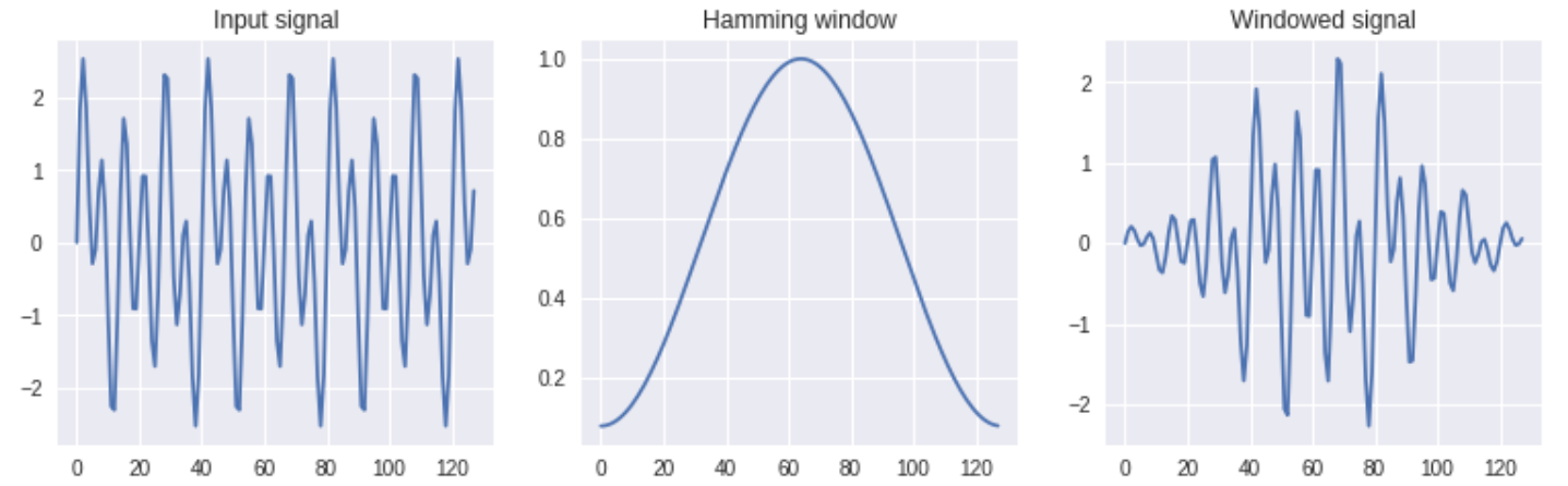
fig = plt.figure(figsize = (13, 8))

ax1 = fig.add_subplot(2, 3, 1)
ax1.plot(sig)
ax1.set_title('Input signal')

ax2 = fig.add_subplot(2, 3, 2)
ax2.plot(win)
ax2.set_title('Hamming window')

ax3 = fig.add_subplot(2, 3, 3)
ax3.plot(win * sig)
ax3.set_title('Windowed signal')

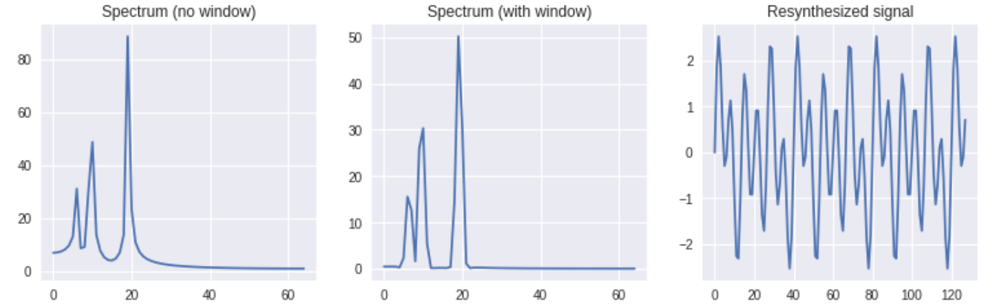
ax4 = fig.add_subplot(2, 3, 4)
ax4.plot(spec_nw)
ax4.set_title('Spectrum (no window)')

ax5 = fig.add_subplot(2, 3, 5)
ax5.plot(spec)
ax5.set_title('Spectrum (with window)')

ax6 = fig.add_subplot(2, 3, 6)
ax6.plot(resyn_sig)
ax6.set_title('Resynthesized signal')

plt.show()

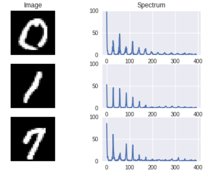
サンプルコード 2

frame_length = 28*28 

indices = np.random.choice(1000, 3)
signals = mnist.train.images[indices]
window = tf.contrib.signal.hamming_window(frame_length) 

signals_f = tf.fft(tf.cast(signals * window, tf.complex64))
half_spectrum = tf.abs(signals_f[:, : frame_length//2 + 1])

with tf.Session() as sess:
  spectrum = sess.run(half_spectrum)
  
fig = plt.figure(figsize = (7, 5))

ax1 = fig.add_subplot(3, 2, 1)
ax1.imshow(np.reshape(signals[0], [28, 28]), cmap = 'gray')
ax1.set_title('Image')
ax1.set_axis_off()

ax2 = fig.add_subplot(3, 2, 2)
ax2.plot(spectrum[0])
ax2.set_ylim(0, 100)
ax2.set_title('Spectrum')

ax3 = fig.add_subplot(3, 2, 3)
ax3.imshow(np.reshape(signals[1], [28, 28]), cmap = 'gray')
# ax3.set_title('Image')
ax3.set_axis_off()

ax4 = fig.add_subplot(3, 2, 4)
ax4.plot(spectrum[1])
ax4.set_ylim(0, 100)
# ax4.set_title('Spectrum')

ax5 = fig.add_subplot(3, 2, 5)
ax5.imshow(np.reshape(signals[2], [28, 28]), cmap = 'gray')
# ax5.set_title('Image')
ax5.set_axis_off()

ax6 = fig.add_subplot(3, 2, 6)
ax6.plot(spectrum[2])
ax6.set_ylim(0, 100)
# ax6.set_title('Spectrum')

plt.show()

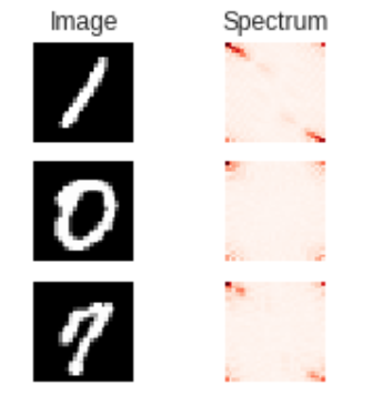
サンプルコード 3

frame_length = 28

indices = np.random.choice(1000, 3)
signals = np.reshape(mnist.train.images[indices], [-1, frame_length, frame_length])
# window = tf.contrib.signal.hamming_window(frame_length) 

signals_f = tf.fft2d(tf.cast(signals, tf.complex64))
spectrum = tf.abs(signals_f) / frame_length ** 2

with tf.Session() as sess:
  spectrum = sess.run(spectrum)
  
fig = plt.figure(figsize = (3, 3))

ax1 = fig.add_subplot(3, 2, 1)
ax1.imshow(np.reshape(signals[0], [28, 28]), cmap = 'gray')
ax1.set_title('Image')
ax1.set_axis_off()

ax2 = fig.add_subplot(3, 2, 2)
ax2.imshow(np.reshape(spectrum[0], [28, 28]), cmap = 'Reds')
ax2.set_title('Spectrum')
ax2.set_axis_off()

ax3 = fig.add_subplot(3, 2, 3)
ax3.imshow(np.reshape(signals[1], [28, 28]), cmap = 'gray')
ax3.set_axis_off()

ax4 = fig.add_subplot(3, 2, 4)
ax4.imshow(np.reshape(spectrum[1], [28, 28]), cmap = 'Reds')
ax4.set_axis_off()

ax5 = fig.add_subplot(3, 2, 5)
ax5.imshow(np.reshape(signals[2], [28, 28]), cmap = 'gray')
ax5.set_axis_off()

ax6 = fig.add_subplot(3, 2, 6)
ax6.imshow(np.reshape(spectrum[2], [28, 28]), cmap = 'Reds')
ax6.set_axis_off()

plt.show()

サンプルコード 4

fs = 800
frame_length = 128
frame_step = 32

a_1 = 0.5
a_2 = 1.0
a_3 = 1.5
f_1 = 40
f_2 = 60
f_3 = 120

sine_1 = a_1 * np.sin(2.0 * np.pi * np.arange(frame_length) * f_1 / fs)
sine_2 = a_2 * np.sin(2.0 * np.pi * np.arange(frame_length) * f_2 / fs)
sine_3 = a_3 * np.sin(2.0 * np.pi * np.arange(frame_length) * f_3 / fs)

signal_1 = tf.convert_to_tensor(sine_1 + sine_2 + sine_3, dtype = tf.float32)

a_4 = 1.5
a_5 = 1.0
a_6 = 0.5
f_4 = 50
f_5 = 100
f_6 = 150

sine_4 = a_4 * np.sin(2.0 * np.pi * np.arange(frame_length) * f_4 / fs)
sine_5 = a_5 * np.sin(2.0 * np.pi * np.arange(frame_length) * f_5 / fs)
sine_6 = a_6 * np.sin(2.0 * np.pi * np.arange(frame_length) * f_6 / fs)

signal_2 = tf.convert_to_tensor(sine_4 + sine_5 + sine_6, dtype = tf.float32)

signals = tf.concat([signal_1, signal_2], axis = 0)

window = tf.contrib.signal.hann_window(frame_length) 

frames = tf.contrib.signal.frame(signals, frame_length = frame_length, frame_step = frame_step)
windowed_frames = window * frames

stfts = tf.contrib.signal.stft(signals, frame_length = frame_length, frame_step = frame_step, \
                               fft_length = frame_length)
magnitude_spectrograms = tf.abs(stfts)

# print (signals)
# print (frames)
# print (stfts)
# print (magnitude_spectrograms)

with tf.Session() as sess:
  signals = sess.run(signals)
  frames = sess.run(frames)
  magnitude_spectrograms = sess.run(magnitude_spectrograms)

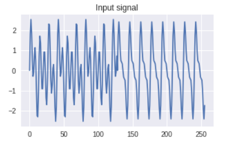
fig_0 = plt.figure(figsize = (5, 3))

ax1 = fig_0.add_subplot(1, 1, 1)
ax1.plot(signals)
ax1.set_title('Input signal')


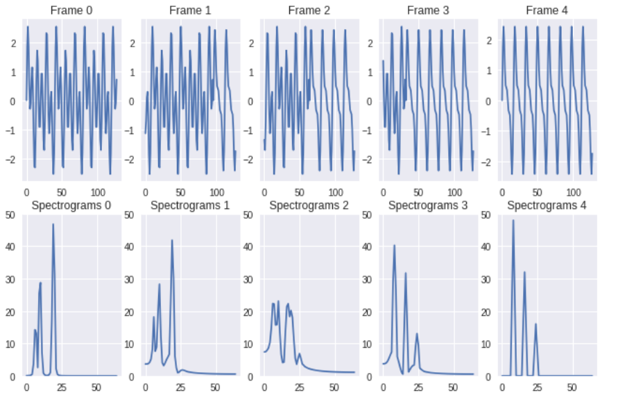
fig = plt.figure(figsize = (11, 7))

ax2 = fig.add_subplot(2, 5, 1)
ax2.plot(frames[0])
ax2.set_title('Frame 0')

ax3 = fig.add_subplot(2, 5, 2)
ax3.plot(frames[1])
ax3.set_title('Frame 1')

ax4 = fig.add_subplot(2, 5, 3)
ax4.plot(frames[2])
ax4.set_title('Frame 2')

ax5 = fig.add_subplot(2, 5, 4)
ax5.plot(frames[3])
ax5.set_title('Frame 3')

ax6 = fig.add_subplot(2, 5, 5)
ax6.plot(frames[4])
ax6.set_title('Frame 4')

ax7 = fig.add_subplot(2, 5, 6)
ax7.plot(magnitude_spectrograms[0])
ax7.set_ylim(0, 50)
ax7.set_title('Spectrograms 0')

ax8 = fig.add_subplot(2, 5, 7)
ax8.plot(magnitude_spectrograms[1])
ax8.set_ylim(0, 50)
ax8.set_title('Spectrograms 1')

ax9 = fig.add_subplot(2, 5, 8)
ax9.plot(magnitude_spectrograms[2])
ax9.set_ylim(0, 50)
ax9.set_title('Spectrograms 2')

ax10 = fig.add_subplot(2, 5, 9)
ax10.plot(magnitude_spectrograms[3])
ax10.set_ylim(0, 50)
ax10.set_title('Spectrograms 3')

ax11 = fig.add_subplot(2, 5, 10)
ax11.plot(magnitude_spectrograms[4])
ax11.set_ylim(0, 50)
ax11.set_title('Spectrograms 4')

plt.show()