2024/4/12に翔泳社よりApache Spark徹底入門を出版します!
書籍のサンプルノートブックをウォークスルーしていきます。Python/Chapter10/10-8 K-Meansとなります。
翻訳ノートブックのリポジトリはこちら。
ノートブックはこちら
このノートブックでは、データをクラスタリングするためにK-Meansを使用します。ラベル(Irisのタイプ)を持つIrisデータセットを使用しますが、トレーニングするために使用するのではなく、モデルの評価のためにラベルだけを使用します。
最後には、分散環境でどのように実装されているのかを見ていきます。
from sklearn.datasets import load_iris
import pandas as pd

# sklearnからデータセットをロードし、Sparkデータフレームに変換
iris = load_iris()
iris_pd = pd.concat([pd.DataFrame(iris.data, columns=iris.feature_names), pd.DataFrame(iris.target, columns=["label"])], axis=1)
irisDF = spark.createDataFrame(iris_pd)
display(irisDF)

"特徴量"として4つの値があることに注意してください。(可視化できるように)これらを2つの値に削減し、DenseVectorに変換します。これを行うためにはVectorAssemblerを使用します。
from pyspark.ml.feature import VectorAssembler

vecAssembler = VectorAssembler(inputCols=["sepal length (cm)", "sepal width (cm)"], outputCol="features")
irisTwoFeaturesDF = vecAssembler.transform(irisDF)
display(irisTwoFeaturesDF)

from pyspark.ml.clustering import KMeans

kmeans = KMeans(k=3, seed=221, maxIter=20)

# estimatorのfitを呼び出し、irisTwoFeaturesDFを入力
model = kmeans.fit(irisTwoFeaturesDF)

# KMeansModelからclusterCentersを取得
centers = model.clusterCenters()

# クラスターの予測結果を追加することでデータフレームを変換するためにモデルを使用
transformedDF = model.transform(irisTwoFeaturesDF)

print(centers)
[array([5.00392157, 3.40980392]), array([5.8, 2.7]), array([6.82391304, 3.07826087])]
イテレーションの数を変えてフィッティングします。
modelCenters = []
iterations = [0, 2, 4, 7, 10, 20]
for i in iterations:
    kmeans = KMeans(k=3, seed=221, maxIter=i)
    model = kmeans.fit(irisTwoFeaturesDF)
    modelCenters.append(model.clusterCenters())
print("modelCenters:")
for centroids in modelCenters:
  print(centroids)
modelCenters:
[array([4.87017544, 3.44561404]), array([6.34146341, 3.03170732]), array([7.42727273, 2.88181818])]
[array([5.01403509, 3.3122807 ]), array([6.128     , 2.84533333]), array([7.28333333, 3.13333333])]
[array([5.01403509, 3.3122807 ]), array([6.03846154, 2.81076923]), array([7.07857143, 3.11071429])]
[array([5.01428571, 3.33571429]), array([5.97 , 2.785]), array([6.98529412, 3.07941176])]
[array([5.01428571, 3.33571429]), array([5.93090909, 2.75272727]), array([6.91025641, 3.08717949])]
[array([5.00392157, 3.40980392]), array([5.8, 2.7]), array([6.82391304, 3.07826087])]
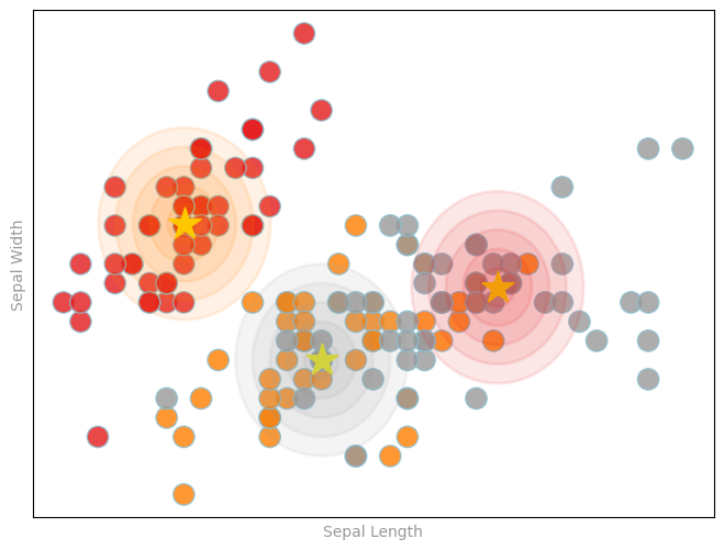
データのtrueラベルに対してクラスタリングがどの程度のパフォーマンスであるのかを可視化しましょう。
覚えておいてください: K-meansではトレーニングの際にtrueラベルは使用しませんが、評価に使用することはできます。
こちらでは、星マークがクラスターの中心です。
import matplotlib.pyplot as plt
import matplotlib.cm as cm
import numpy as np

def prepareSubplot(xticks, yticks, figsize=(10.5, 6), hideLabels=False, gridColor='#999999',
                gridWidth=1.0, subplots=(1, 1)):
    """プロットレイアウト生成のテンプレート"""
    plt.close()
    fig, axList = plt.subplots(subplots[0], subplots[1], figsize=figsize, facecolor='white',
                               edgecolor='white')
    if not isinstance(axList, np.ndarray):
        axList = np.array([axList])

    for ax in axList.flatten():
        ax.axes.tick_params(labelcolor='#999999', labelsize='10')
        for axis, ticks in [(ax.get_xaxis(), xticks), (ax.get_yaxis(), yticks)]:
            axis.set_ticks_position('none')
            axis.set_ticks(ticks)
            axis.label.set_color('#999999')
            if hideLabels: axis.set_ticklabels([])
        ax.grid(color=gridColor, linewidth=gridWidth, linestyle='-')
        map(lambda position: ax.spines[position].set_visible(False), ['bottom', 'top', 'left', 'right'])

    if axList.size == 1:
        axList = axList[0]  # 通常のプロットには単一のaxesオブジェクトを返却
    return fig, axList
data = irisTwoFeaturesDF.select("features", "label").collect()
features, labels = zip(*data)

x, y = zip(*features)
centers = modelCenters[5]
centroidX, centroidY = zip(*centers)
colorMap = 'Set1'  # was 'Set2', 'Set1', 'Dark2', 'winter'

fig, ax = prepareSubplot(np.arange(-1, 1.1, .4), np.arange(-1, 1.1, .4), figsize=(8,6))
plt.scatter(x, y, s=14**2, c=labels, edgecolors='#8cbfd0', alpha=0.80, cmap=colorMap)
plt.scatter(centroidX, centroidY, s=22**2, marker='*', c='yellow')
cmap = cm.get_cmap(colorMap)

colorIndex = [.5, .99, .0]
for i, (x,y) in enumerate(centers):
    print(cmap(colorIndex[i]))
    for size in [.10, .20, .30, .40, .50]:
        circle1=plt.Circle((x,y),size,color=cmap(colorIndex[i]), alpha=.10, linewidth=2)
        ax.add_artist(circle1)

ax.set_xlabel('Sepal Length'), ax.set_ylabel('Sepal Width')
display(fig)
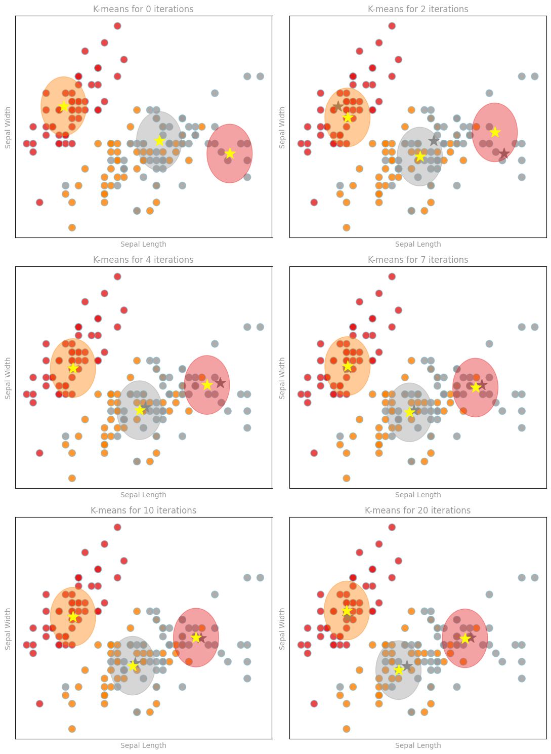
それぞれのイテレーションでクラスターのオーバーレイを確認することに加え、イテレーションごとにクラスターの中心がどのように動くのかを確認することができます(イテレーションが少ない場合に結果がどのようなものになるのかも確認できます)。
x, y = zip(*features)

oldCentroidX, oldCentroidY = None, None

fig, axList = prepareSubplot(np.arange(-1, 1.1, .4), np.arange(-1, 1.1, .4), figsize=(11, 15),
                             subplots=(3, 2))
axList = axList.flatten()

for i,ax in enumerate(axList[:]):
    ax.set_title('K-means for {0} iterations'.format(iterations[i]), color='#999999')
    centroids = modelCenters[i]
    centroidX, centroidY = zip(*centroids)

    ax.scatter(x, y, s=10**2, c=labels, edgecolors='#8cbfd0', alpha=0.80, cmap=colorMap, zorder=0)
    ax.scatter(centroidX, centroidY, s=16**2, marker='*', c='yellow', zorder=2)
    if oldCentroidX and oldCentroidY:
      ax.scatter(oldCentroidX, oldCentroidY, s=16**2, marker='*', c='grey', zorder=1)
    cmap = cm.get_cmap(colorMap)

    colorIndex = [.5, .99, 0.]
    for i, (x1,y1) in enumerate(centroids):
      print(cmap(colorIndex[i]))
      circle1=plt.Circle((x1,y1),.35,color=cmap(colorIndex[i]), alpha=.40)
      ax.add_artist(circle1)

    ax.set_xlabel('Sepal Length'), ax.set_ylabel('Sepal Width')
    oldCentroidX, oldCentroidY = centroidX, centroidY

plt.tight_layout()

display(fig)
(1.0, 0.4980392156862745, 0.0, 1.0)
(0.6, 0.6, 0.6, 1.0)
(0.8941176470588236, 0.10196078431372549, 0.10980392156862745, 1.0)
(1.0, 0.4980392156862745, 0.0, 1.0)
(0.6, 0.6, 0.6, 1.0)
(0.8941176470588236, 0.10196078431372549, 0.10980392156862745, 1.0)
(1.0, 0.4980392156862745, 0.0, 1.0)
(0.6, 0.6, 0.6, 1.0)
(0.8941176470588236, 0.10196078431372549, 0.10980392156862745, 1.0)
(1.0, 0.4980392156862745, 0.0, 1.0)
(0.6, 0.6, 0.6, 1.0)
(0.8941176470588236, 0.10196078431372549, 0.10980392156862745, 1.0)
(1.0, 0.4980392156862745, 0.0, 1.0)
(0.6, 0.6, 0.6, 1.0)
(0.8941176470588236, 0.10196078431372549, 0.10980392156862745, 1.0)
(1.0, 0.4980392156862745, 0.0, 1.0)
(0.6, 0.6, 0.6, 1.0)
(0.8941176470588236, 0.10196078431372549, 0.10980392156862745, 1.0)
それでは、分散環境では何が起きているのかを見てみましょう。
Mapステージ
Mapステージでは、クラスターに対してポイントが割り当てられます。

Reduceステージ
Reduceステージでは、クラスターの中心を選択し、クラスターに属するポイントのセントロイドが新たな中心となります。

通信
-
Map: クラスターへのポイントの割り当て -> P台のワーカーにk個のクラスターの中心を送信します。
-
Reduce: クラスターの中心の選択 -> n個のポイントからk個のクラスターの中心に集約、しかし最初にそれぞれのワーカー内で集計可能です!
中心とポイントはd次元のベクトルとなります。
トータルの通信量は: O(kdP)
通信量はポイントの数nに依存しません!
通信量は以下に依存します:
- ワーカーの台数P -> ツリー集計による並列化
- 次元数d -> dが高い場合、K-Meansは失敗することがあります
- クラスター数k -> 避けることは困難です

Take Aways
分散MLアルゴリズムを設計/選択する際には:
- コミュニケーションが鍵となります!
- お使いのデータ/モデルの次元数とどれだけのデータを必要とするのかを検討します
- データのパーティショニングと構成が重要となります。