Automating GIS Processes 2024 写経 Lesson 7 Processing and Analysis of Raster Data（２）

前回 の続きです。

Raster reclassification

Raster reclassification is another common procedure with raster dataset. Raster reclassification is the process of assigning new values to the pixels of a raster dataset based on their existing values. This is often used to simplify or categorize continuous data, such as elevation or land cover, into distinct classes. For example, in an elevation map, reclassification can group different elevation ranges into categories like “low”, “medium”, and “high” altitude, making it easier to analyze or visualize the data for specific applications such as hazard assessment or land management.

let’s first have a look at the range of values (altitudes) in our raster data:

ラスタの再分類はラスタのデータを取りあつかう、一般的な手段のひとつです。既存の値に基づいて、新しい値をラスタのデータセットに割り当てます。
これは、継続的なデータ、例えば標高や土地被覆（地表面を覆っているもの）を、単純化、もしくは、独立した分類の箱（class）に仕分けする目的で、よく使われます。
例えば、ある標高のマップで、再分類により、異なる標高を、"低"・"中"・"高"の異なる標高の幅でグループ化できます、これにより、有害性評価や土地保全といった用途におけて、データ分析や可視化がしやすくなります。

では、幅の値について、見てみましょう。

# Check the data range
print(clipped_raster.min().values, clipped_raster.max().values)

幅の値は、-1.8289999961853027から31.833999633789062に収まっています。

Now we want to reclassify our data using two approaches. First, let’s do it manually using the numpy library. NumPy is a powerful Python library used for numerical and scientific computing. It provides support for large, multi-dimensional arrays and matrices, along with a wide collection of mathematical functions to operate on these arrays efficiently. So basically here, we are treating our pixel values as an Array and do the calculations accordingly.

さて、2つのアプローチでデータを再分類したいです。
最初に、numpyのライブラリを使って手動でやってみましょう。NumPy は数値や科学的な計算のために使われるパワフルなPythonのライブラリです。配列を効果的に処理する幅広い数学の関数のコレクションによって、大規模、かつ、多次元な配列とマトリックスに対応します。
なので、基本的に、ここではピクセル値を一つのArrayとして計算をします。

Note: An array (such as those created by NumPy) is a multi-dimensional container for data, but it lacks metadata like coordinate labels or attributes. In contrast, an xarray.DataArray enhances the array by adding labeled dimensions, coordinates, and attributes, making it easier to work with multi-dimensional data, especially in geospatial and time-series contexts.

メモ：　一つのArray（Numpyで作られたものなど）は、多次元のデータの入れ物です。しかし、このArrayは座標ラベルや属性のようなメタデータが欠落しています。
一方、xarray.DataArrayは、配列に多次元・座標・属性を与えることができます。これにより、地理空間や時系列のコンテキスト（背景となる情報）を持つ多次元データが処理しやすくなります。

import numpy as np
import xarray as xr
import matplotlib.pyplot as plt

# Define the bins and new class values
bins = [-10, 10, 20, np.inf]  # Bins for elevation
new_values = [1, 2, 3]  # Class values: 1 for Low, 2 for Mid, 3 for High

# Mask out NaN values before reclassification
masked_raster = np.where(~np.isnan(clipped_raster), clipped_raster, np.nan)

# Apply the reclassification
reclassified_raster = np.digitize(masked_raster, bins, right=True)

# Retain NaN values by ensuring they are not reclassified
reclassified_raster = np.where(~np.isnan(clipped_raster), reclassified_raster, np.nan)

# Convert to an xarray DataArray
reclassified_raster = xr.DataArray(
    reclassified_raster,
    dims=clipped_raster.dims,  # Keep the same dimensions
    coords=clipped_raster.coords,  # Retain the spatial coordinates
    attrs=clipped_raster.attrs  # Preserve the original attributes
)

# Plot using xarray's plot method
plot = reclassified_raster.plot(cmap=plt.matplotlib.colors.ListedColormap(['blue', 'green', 'brown']))

# Set only the ticks [1, 2, 3] on the colorbar
colorbar = plot.colorbar
colorbar.set_ticks([1, 2, 3])
colorbar.set_ticklabels(['Low', 'Mid', 'High'])  # Rename the labels
colorbar.set_label("Elevation class")

plt.title("Classified elevation")
plt.show()

Note: When using np.digitize(), the function returns indices of the bins, starting from 1. This means the output will not directly contain the desired reclassified values. To map the bin indices to the actual values, you need to create a mapping, such as using a list comprehension to convert the indices into the specified new values. Don’t forget to subtract 1 from the indices because Python lists are zero-indexed, while np.digitize() starts indexing at 1.

メモ：：np.digitize()関数は、ビンのインデックスの配列を返しますが、１オリジンです。
これは、出力が一発で意図する分類値にならないということです。
ビンのインデックスを実際の値に割り当てるため、マッピングをする必要があります。例えば、インデックスの配列を特定の値に置き換える内包表記のような。
インデックスの配列から1を減算することを忘れないでください。　Pythonのリストは０オリジンですが、np.digitize()関数の戻り値１オリジンなので。

ここなんだかよくわからないので、ちょっと試してみます。
ビンは変えていません。なお、4ビン目のnp.infは、無限大です。

import numpy as np
import xarray as xr
import matplotlib.pyplot as plt

# Define the bins and new class values
bins = [-10, 10, 20, np.inf]  # Bins for elevation

# Mask out NaN values before reclassification
masked_raster = np.where(~np.isnan(clipped_raster), clipped_raster, np.nan)

# Apply the reclassification
print(np.digitize(masked_raster, bins, right=True).min())
print(np.digitize(masked_raster, bins, right=True).max())

np.digitize()関数の戻り値は、１～４なので、１オリジンです。

# Plot using xarray's plot method
reclassified_raster.plot(cmap=plt.matplotlib.colors.ListedColormap(['blue', 'green', 'brown']))

カラーバーの値は、１～３（無限大は表現されない）となっています。やはり1オリジンです。

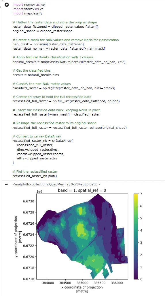
We can use the mapclassify library which we learned about in Lesson 4, to reclassify our raster. Let’s Try NaturalBreaks method here.

レッスン４で学んだ、ラスタを再分類できるmapclassifyライブラリを使うことができます。
ビン数７の自然分類（NaturalBreaks）でやってみます。

import numpy as np
import xarray as xr
import mapclassify

# Flatten the raster data and store the original shape
raster_data_flattened = clipped_raster.values.flatten()
original_shape = clipped_raster.shape

# Create a mask for NaN values and remove NaNs for classification
nan_mask = np.isnan(raster_data_flattened)
raster_data_no_nan = raster_data_flattened[~nan_mask]

# Apply Natural Breaks classification with 7 classes
natural_breaks = mapclassify.NaturalBreaks(raster_data_no_nan, k=7)

# Get the classified bins
breaks = natural_breaks.bins

# Classify the non-NaN raster values
classified_raster = np.digitize(raster_data_no_nan, bins=breaks)

# Create an array to hold the full reclassified data
reclassified_full_raster = np.full_like(raster_data_flattened, np.nan)

# Insert the classified data back, keeping NaNs in place
reclassified_full_raster[~nan_mask] = classified_raster

# Reshape the reclassified raster to its original shape
reclassified_full_raster = reclassified_full_raster.reshape(original_shape)

# Convert to xarray DataArray
reclassified_raster_nb = xr.DataArray(
    reclassified_full_raster,
    dims=clipped_raster.dims,
    coords=clipped_raster.coords,
    attrs=clipped_raster.attrs
)

# Plot the reclassified raster
reclassified_raster_nb.plot()

Raster reclassification and NaN values When reclassifying raster data, it’s crucial to handle null values (NaNs) carefully. If not properly masked, NaN values can be incorrectly classified, leading to erroneous results. Always ensure that NaN values are preserved or treated appropriately to avoid classification issues and maintain accurate analysis.

ラスタを再分類するときは、NaN値（非数値）を注意深く扱う必要があります。適切にマスクがかかっていないと、NaN値が原因となる誤った分類になり、誤った結果となります。
分類で問題が起こることを避け、正確な分類を維持するため、NaN値が適切に保存されているか、処理されているかをいつも確かめましょう。

Slope analysis

Slope analysis is a key terrain analysis technique used in GIS and spatial analysis to measure the steepness or incline of the terrain at any given point. It is calculated by examining the rate of change in elevation between neighboring pixels in a digital elevation model (DEM). Slope analysis helps identify areas with steep gradients, which is useful in applications like land-use planning, erosion risk assessment, hydrological modeling, and infrastructure development. The slope is typically expressed in degrees or as a percentage.

Of course, we can perform slope analysis anywhere, including on the Helsinki city center raster we worked with earlier. However, for this course’s purpose, it will be more interesting to calculate it for an area with more elevation variation. Since Finland is generally quite flat, we need to look further north to find terrain that is more elevation-wise interesting for slope analysis. For this purpose, we are heading to Ylläs in Lapland, located in the northern part of Finland. Ylläs is a fell, or mountainous hill, and offers more diverse elevation changes, making it ideal for our slope analysis!

傾斜分析は、GISや空間分析で使われ、とある地形の傾きの度合いを計測するための主要な分析手法です。
数値標高モデル（DEM）の隣接するピクセル間の標高の差の度合いを検査することで計算されます。
傾斜分析は急勾配の場所を特定する助けになります。そして、それは、土地利用計画、土地の浸食のリスク評価、水文モデリング（水循環のモデリング）・インフラ整備などの役に立ちます。
傾斜は一般的に度もしくはパーセントで表現されます。

もちろん、私たちはどこでも傾斜分析ができます。先ほど扱ったヘルシンキの市街地のラスタであっても。
しかし、このコースの目的を考えると、もっと標高のバリエーションがある場所でそれをするほうが興味深くなるでしょう。
フィンランドはかなりフラットなので、もっと傾斜分析をするうえで面白い地形をさがすため、より北に向かいます。
目的を考え、フィンランド北部、ラップランドのユッラスを目指します。ユッラスは山、あるいは丘陵で、多様な傾斜の変化があり、傾斜分析にはうってつけです。

About Ylläs

Ylläs is one of the highest fells in Finland, standing at 718 meters. It is located in the Pallas-Yllästunturi National Park and is a popular destination for outdoor activities such as hiking and skiing. Ylläs is known for its stunning natural landscapes, including vast forests, pristine lakes, and dramatic fells that rise above the surrounding terrain.

ユッラスはフィンランドにおいても最も高い山の一つであり、標高718メートルです。
パッラス・ユッラストゥントゥリ国立公園に位置し、ハイキングやスキーといったアウトドアのアクティビティの目的地として人気があります。
ユッラスは風光明媚な場所として有名で、広大な森林・手つかずの湖沼・周囲の地形よりも高いドラマチックな山々があります。

The raster we will be working with is from the same source as the previous ones, provided by the National Land Survey of Finland, but from a different tile (U4234). We will calculate the slope using our clipped elevation raster. The slope at each point is derived by determining the rate of change in elevation between neighboring cells in the raster. This is done by:

1. Gradient Calculation: We use the elevation differences between adjacent cells in both the x (horizontal) and y (vertical) directions. The gradient represents how quickly elevation changes in these directions.
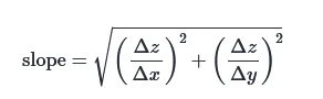
2. Slope Formula: The slope is calculated by combining these gradients using the Pythagorean theorem:
   
   where Delta z is the change in elevation, and Delta x and Delta y are the distances between the cells in the x and y directions.
3. Final Slope Values: The result is often expressed in degrees or as a percentage, with steeper areas showing higher slope values. We use degrees here.

私たちが扱っているラスタのデータソースは前回と同じで、National Land Survey of Finland によって提供されたものですが、タイルは違います。（U4234）
私たちはクリップされた標高のラスタを使って、傾斜を計算します。各点の傾斜は、ラスタの隣のセルの標高との変化の割合によって変わります。これは以下の通りです。

1. 勾配計算: 隣接するセルとのx（水平）方向・y（垂直）方向それぞれの標高差／距離。勾配は高さの変化がどのぐらい急なのかを示します。

2. 傾斜の公式: ピタゴラスの定理を使って、x方向とy方向の勾配を合成して算出されます:
   
   Δzは高さの変化で、ΔxとΔyはそれぞれ、x方向、y方向のセル間の距離。
   （上図ではΔzが２回登場するが、左側はΔzₓ、右側はΔzᵧです。）

3. 最終的な傾斜の値: 結果は、度もしくはパーセントで、より急な範囲がより高い傾斜の値として表示されます。今回は度を使います。

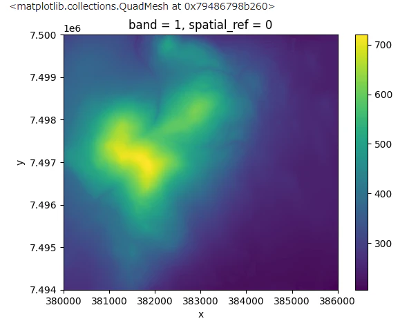
では、まず、タイルを読み込み、単純にプロットしてみます。

yllas_dem = rioxarray.open_rasterio('data/U4234A.tif')
yllas_dem.plot()

次に、傾斜を求めます。

# Get the pixel resolution
xres = yllas_dem.rio.resolution()[0]  # Resolution in x direction (longitude)
yres = yllas_dem.rio.resolution()[1]  # Resolution in y direction (latitude)

# Calculate gradients in the x and y directions
dzdx = yllas_dem.differentiate(coord='x') / xres  # Gradient in the x direction
dzdy = yllas_dem.differentiate(coord='y') / yres  # Gradient in the y direction

# Calculate the slope (in degrees)
slope = np.sqrt(dzdx**2 + dzdy**2)
slope = np.arctan(slope) * (180 / np.pi) # 配の大きさ（= tanθ に相当）を arctan で角度（ラジアン）に変換し、度に変換

# Update the attributes to reflect that this is a slope raster
slope.attrs['long_name'] = 'Slope'
slope.attrs['units'] = 'degrees'

これだけだとよくわからないので、slopeの中身してみましょう。

Attributesとして、long_nameとunitsを設定しています。こは、プロットしたときのカラーバーのタイトルになります。

Now let’s plot our Slope raster.

では、傾斜のラスタをプロットしてみましょう。

# Plot the slope raster
plt.figure(figsize=(10, 8))
slope.plot(cmap='terrain', add_colorbar=True)
plt.title("Slope Map (Degrees)")
plt.xlabel("X Coordinate")
plt.ylabel("Y Coordinate")
plt.show()

やはり、標高とはだいぶ違いますね。

長くなったので、ここまでにします。