Automating GIS Processes 2024 写経 Lesson 7 Exploring raster data in Python（1）

Raster data consists of rows and columns of cells or pixels, with each cell representing a single value. This type of data is often thought of as images, although raster datasets can be stored in various formats such as ASCII text files or Binary Large Objects (BLOBs) within databases.

ラスタデータはセルかピクセルの行列で構成されていて、各々のセルは一つだけ値を持っています。
このような型のデータは、しばしば画像として考えられます。例えば、アスキーのテキストファイルやデータベースにある**バイナリ・ラージ・オブジェクト（BLOB）**のように、ラスタのデータセットは、さまざまなフォーマットに格納されるにもかかわらず。

Raster data represents the world as a grid of equally sized cells or pixels, where each cell has a value representing information, such as temperature, elevation, or land cover. There are two primary ways of working with raster data:

• Single-band raster: Each pixel has one value (e.g., elevation or temperature).
• Multiband raster: Each pixel has multiple values (e.g., Red, Green, and Blue bands in satellite imagery).

ラスタデータは世界を同じサイズのセルかピクセルのグリッドとして表現します。そこで各々のセルは情報を表現する値を持ちます、例えば、温度、標高、ランドローバー（地表面の要素）などです。ラスタデータを扱う２つの主要な方法があります。

• シングルバンドラスタ（帯域がひとつのラスタ）：各々のピクセルは一つの値を持ちます（例えば、標高や温度）
• マルチバンドラスタ（帯域が複数のラスタ）：各々のピクセルは複数の値を持ちます（例えば、衛星画像の赤色、緑色、青色の帯域）

A key characterestic of any raster data is its Resolution. Resolution refers to the ground distance that each cell represents. For example, if the resolution is two meters, each cell corresponds to an area two meters by two meters. A raster dataset with higher resolution can show more detail, but it will also have larger file sizes.

どのラスタデータにおいてもキーとなる特性はその解像度です。
解像度は各々のセルが表現する地面の距離に関連します。例えば、解像度が２メートルの場合、各々のセルは2メートル×2メートルの面積、となります。
高解像度のラスタのデータセットはより詳細な表示ができます。しかし、そのラスタのファイルサイズはより大きくなります。

Raster data can be stored in a variety of formats, some of the more common ones include:

• TIFF (Tagged Image File Format): This is the most common geospatial raster format due to its flexibility. It allows for storage of multiple bands, metadata, and internal compression. However, TIFF files can sometimes be incompatible across software.
• JPEG, GIF, BMP, PNG: These formats are more suitable for images used in presentations or online applications. While common, they are not as robust for storing geospatial data due to lack of metadata support.
• ASCII Grid: This format is often used for storing elevation data as simple text files, with spatial information stored in a header.

ラスタデータはいろいろなフォーマットで保存されます。いくつかのより一般的なものは：

• TIFF (Tagged Image File Format)：その柔軟性のおかげで、もっとも人気のある地理空間のラスタフォーマット。マルチバンド、メタデータ、自己圧縮での保存が可能、しかし、ソフトウェア間で互換性がない場合があります。
• JPEG, GIF, BMP, PNG：これらのフォーマットは、プレゼンテーションやオンラインアプリケーションで使われてる画像に適している。だがしかし、メタデータのサポート不足という点で、地理空間データの保存については、あまり堅牢でない
• ASCII Grid：しばしば、空間情報がヘッダに格納された単純なテキストファイルに標高データを保存するために使われる

Raster data analysis with Python

In this lesson we will learn to perform raster GIS analysis using a number of Python libraries. You’ll learn how to read, manipulate, analyze, and visualize raster data using xarray, rioxarray, and xarray-spatial.

• xarray: A powerful library for working with labeled, multi-dimensional arrays in Python. It is particularly useful for handling scientific data, including time series and spatial data.
• rioxarray: An extension of xarray designed for geospatial raster data operations. It builds on top of rasterio to handle reading and writing raster formats like GeoTIFF, working with CRS (Coordinate Reference Systems), and performing GIS-specific tasks like reprojection. This combination allows for easy manipulation of spatial data in a highly efficient manner.
• xarray-spatial: A high-performance spatial analysis library that works with xarray to perform raster-based spatial analysis tasks such as terrain analysis, focal operations, and zonal statistics. It is designed for fast processing of large datasets.

このレッスンでは、いくつかのPythonライブラリを使って、ラスタのGIS分析のやり方を学びます。
xarray、rioxarray、xarray-spatialによるラスタデータの読み方、計算の仕方、分析の仕方、表示の仕方を学びます。

• xarray：ラベル付けされた、多次元の配列上で動作するパワフルなPythonライブラリ
• rioxarray：xarrayの拡張で、地理空間ラスタデータの操作のためにデザインされている。rasterio上で作成され、ラスタフォーマットをGeoTIFFのように読み書きすることができ、CRS（座標参照系）に対応し、再投影のようなGIS特有のタスクを行う。
• xarray-spatial：高パフォーマンスの空間分析ライブラリ、xarrayとあわせて、地形分析、焦点演算、ゾーン統計のような、ラスタをベースとする空間分析を行う。大きなデータセットを高速で処理するようにデザインされている。

These libraries are closely related to rasterio, which is the core library for handling raster data formats. rasterio is built on the GDAL (Geospatial Data Abstraction Library) and provides efficient, low-level input and output operations for raster data, supporting various formats like GeoTIFF, PNG, and JPEG. It allows you to read and write raster files, access pixel values, manage CRS, and perform raster data manipulation.

これらのライブラリはrasterioとかなりの関連があります。rasterioはラスタデータのフォーマットを扱ううえで、核となるライブラリです。
rasterioはGDAL(地理空間データ抽象化ライブラリ)上で作られ、ラスタデータの効率性な低レベルの（OSの機能を使った）入出力操作を提供し、GIFF、PNG、JPEGのようなさまざまなフォーマットをサポートします。このライブラリにより、ラスタのファイルの読み書き、ピクセル値へのアクセス、CRSの管理、ラスタデータの操作が可能になります。

rioxarray uses rasterio under the hood to handle the actual reading and writing of raster files. The flexibility of xarray combined with rasterio’s capabilities provides us with useful tools for analysis of raster data.

In this part of our raster lesson, we will learn how to:

• Import and read raster data in Python
• Visualize raster data

rioxarrayは、ラスタのファイルを実際に読み書きするために、内部でrasterioを使います。
rasterioの能力をもつxarrayの柔軟性は、ラスタデータの分析に役立つツールを提供します。

今回のラスタについてのレッスンで、以下の方法を学びます：

• Pythonでラスタデータを読み込む
• ラスタデータを可視化する

Loading raster data

For this lesson, we will work with two raster datasets (and briefly preview an additional one):

• Sentinetl 2 satelite image from Nuuksio national park in Finland. Data is obtained from Copernicus Data Space Ecosystem
• Elevation model data retrieved from National Land Survey of Finland.

このレッスンでは、２つのラスタデータセットを使います。（そして、追加のデータセットのプレビューをします）

• Copernicus Data Space Ecosystemから取得した、センチネル2からの、フィンランドのヌークシオ国立公園（Nuuksio national park）の衛星画像
• National Land Survey of Finlandから取得した標高モデルデータ

Loading Single-Band Raster Data

To load single-band raster data, we use the rioxarray library. rioxarray is built on top of xarray and rasterio. Under the hood, rioxarray utilizes rasterio to handle reading the raster file formats like GeoTIFF. This means that when we import a raster file using rioxarray, it uses rasterio to read the file and load it into an xarray.DataArray structure, making it easy to manipulate, visualize, and analyze the data.

シングルバンドラスタを読み込むために、rioxarrayライブラリを使います。rioxarrayはxarrayとrasterio上で作成されています。GeoTIFFのようなラスタのファイルフォーマットを読み込むために、rioxarrayは、内部でrasterioを使います。

The data we will use here elevation model data provided from National Land Survey of Finland. Let’s start with loading one of the four tiles that we will be working with later during this lesson (L4133A.TIF).

私たちがこのレッスンで使うデータは、National Land Survey of Finlandから提供されたものです。
それでは、４タイルのうち、１つ、このレッスンで使うL4133A.TIFファイルを読み込んでみましょう。

（ファイルは以下にあります。ファイルの拡張子は大文字ではなく、小文字です。）
https://github.com/Automating-GIS-processes/notebooks/tree/main/lesson-7/data

（rioxarrayはインポートされていないため、手動でインポートする必要があります）

! pip install rioxarray

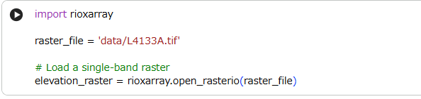
import rioxarray

raster_file = 'data/L4133A.tif'

# Load a single-band raster
elevation_raster = rioxarray.open_rasterio(raster_file)
![image.png](https://qiita-image-store.s3.ap-northeast-1.amazonaws.com/0/4076503/49429759-98c0-42fc-ba18-06d217b5559d.png)

Let’s have a look at the meatdata:

読み込んだファイルのメタデータを見てみましょう。

We can see from the metadata that the raster file contains a single band with dimensions of 3000x3000 pixels, and the pixel values are stored as 32-bit floating point numbers. The coordinates are georeferenced, with x and y representing the spatial extent of the image, and there is a defined fill value of -9999.0 for missing data.

メタデータより、ラスタファイルが3000×3000ピクセルのシングルバンド（band:1）で、ピクセル値は32ビットの浮動小数点（dtype=float32）として保存されていることがわかります。
座標（coordinates）は、画像の空間的広がりを示すxとyで割り当てされて（georeferenced）、欠損がある場合は-9999.0で穴埋めする定義（_FillValue: -9999.0）があります。

Now let’s check the CRS and then make a quick plot of our raster data to see what it looks like.

では、CRSをチェックし、どのように見えるかを確認するために、読み込んだラスタデータを簡単にプロットしてみましょう。

# Checking the CRS of our raster data
elevation_raster.rio.crs

なんだかよくわからないので、CRSをEPSGで表示します。

elevation_raster.rio.crs.to_epsg()

EPGS: 3967は、フィンランドなので、良さそうです。

では、改めて、プロットします。

# Make a quick plot
elevation_raster.plot()

これだけだと、よくわからないですね。。。

Now let’s use numpy library and print some basic raster statistics:

では、numpyライブラリを使って、基本的なラスタの統計情報を出してみましょう。

# Print basic statistics
print(f"Min value: {elevation_raster.min().item()}")
print(f"Max value: {elevation_raster.max().item()}")
print(f"Mean value: {elevation_raster.mean().item()}")
print(f"Median value: {elevation_raster.median().item()}")
print(f"Standard deviation: {elevation_raster.std().item()}")

長くなったので、いったんここまでにします。