はじめに
データ分析や機械学習などに利用できるプログラムとして、Juliaがあると知った。
以下3点のメリットから今後利用することがあるかもしれないので、備忘録として初歩的なことから欲しかった資料をまとめていく。
[1]Pythonと同じようにライブラリを利用できる
[2]実行速度がC言語よりも速い
[3]PythonやC言語と連携することもできる
実行環境
参考資料[1]で構築したVSCにおけるWSL2で実行している。
検証したプログラム
前回まで:
https://qiita.com/svoboda/items/85fc2301b449ba1e5137
Juliaプログラム
main.jl(クリックで展開)
include("read_csv.jl")
include("completion_numeric_data.jl")
include("knn_imputation.jl")

# main 関数
function main()
    # ファイルパスを指定
    file_path = "../data/raw/random_data_100.csv"

    # 関数を呼び出してデータフレームを取得
    hunter_information = read_csv_to_dataframe(file_path)

    # 数値データの欠損値を平均値で補完
    hunter_information = completion_mean(hunter_information, "play_time")

     # 欠損値があるStringデータ項目
    column = "sub_weapon"

    # 説明変数として使いたい列
    features = [:HR, :gender, :area, :main_weapon, :play_time]

    # Stringデータの欠損値をKNNで補完
    hunter_information = fill_missing_data_with_knn(column, hunter_information, features, 5)# Pass 5 as k


    # データフレームを表示
    println(hunter_information)

end

# main 関数を実行
@time begin #実行時間計測用
    main()
end
read_csv.jl(クリックで展開)
using CSV,DataFrames

# CSVを読み取り、データフレームに取り込む
function read_csv_to_dataframe(file_path::String)
    csv_information = CSV.File(file_path) |> DataFrame

    return csv_information
end
completion_numeric_data.jl(クリックで展開)
using Statistics

# データフレーム読み取り、数値データの欠損値を平均値で補完
function completion_mean(data, column)
    #欠損値があるcolumnの平均を導出
    column_mean = mean(skipmissing(data[!,column]))

    # 列 column の欠損値を平均値で埋める
    data[!,column] .= coalesce.(data[!,column], column_mean)

    return data

end
knn_imputation.jl(クリックで展開)
using MLJ
using MLJModelInterface
using NearestNeighborModels
using DataFrames
using CategoricalArrays
using Tables

"""
    fill_missing_data_with_knn(column::String, df::DataFrame, features::Vector{Symbol}, k::Int)

`column` に指定されたカテゴリ列の欠損値を、指定された `features` を使って
K近傍法(KNN)で補完する。

# 引数
- `column` : 補完対象の列名(例: "sub_weapon")
- `df`     : 対象の DataFrame
- `features`: 説明変数として使う列の Symbol 配列(例: [:HR, :gender, ...])
- `k`      : KNNの近傍数(例: 5)

# 戻り値
- 欠損が補完された DataFrame
"""
function fill_missing_data_with_knn(column::String, df::DataFrame, features::Vector{Symbol}, k::Int)
    # 1. 対象列(補完対象)を取得
    y_raw = df[:, column]
    y = convert(CategoricalVector{Union{Missing, String}}, y_raw)
    missing_idx = findall(ismissing, y)

    # 欠損がなければ何もしない
    if isempty(missing_idx)
        println("🔵 欠損は見つかりませんでした: $column")
        return df
    end

    # 2. 説明変数を準備
    X_raw = df[:, features]

    # 3. カテゴリ変数を CategoricalVector に変換(missingありでもOK)
    for col in features
        col_eltype = eltype(X_raw[!, col])
        if col_eltype <: AbstractString || col_eltype <: Union{Missing, AbstractString}
            X_raw[!, col] = convert(CategoricalVector{Union{Missing, String}}, X_raw[!, col])
        end
    end

    # 4. OneHotEncoderでカテゴリ列を数値ベクトルに変換(数値データに変換しないと正常動作できない)
    encoder = OneHotEncoder()
    mach_enc = machine(encoder, X_raw)
    fit!(mach_enc)
    X_encoded_tbl = MLJ.transform(mach_enc, X_raw)  # テーブル形式

    # 5. MLJのKNNは Matrix{Float64} を要求するため明示変換
    X_encoded = Matrix{Float64}(Tables.matrix(X_encoded_tbl))

    # 6. 欠損のない行のみで学習
    observed_idx = findall(!ismissing, y)
    X_obs = DataFrame(X_encoded[observed_idx, :], :auto)
    y_obs = coerce(collect(skipmissing(y[observed_idx])), Multiclass)  # ← missing除去

    # 7. KNNモデルで学習
    knn = KNNClassifier(K=k)
    mach = machine(knn, X_obs, y_obs)
    fit!(mach)

    # 8. 欠損のある行に対して予測
    X_missing = X_encoded[missing_idx, :]
    y_pred = mode.(predict(mach, X_missing))

    # 9. 元のラベル列に補完値を反映
    y[missing_idx] .= y_pred
    df[:, column] = y

    return df
end
結果
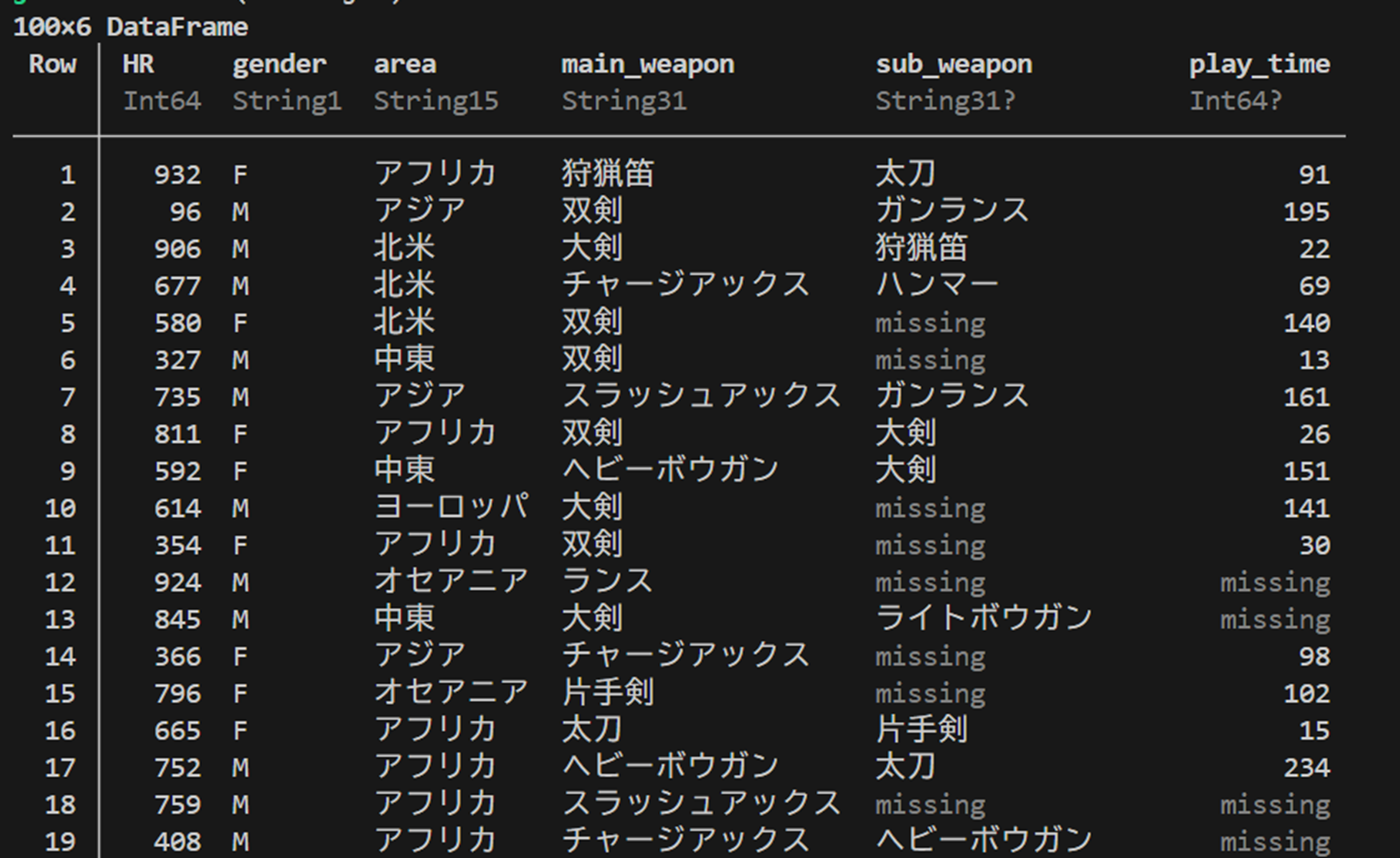
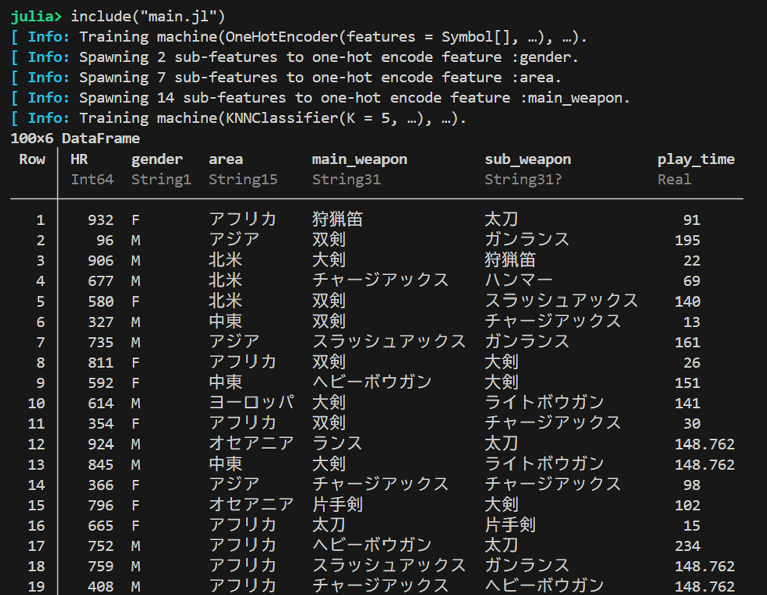
実行結果
1つ目の画像が実行前だが、2つ目の実行画像のように欠損値が補完されていることを確認できた。
速度検証結果
処理時間について以下のような結果となった。
①初回実行時間はいづれも10秒程度でデータ件数による差異はあまりなかった。
②2回目以降の処理時間について、1回目よりも1/10~1/1000に小さくなる。
③2回目以降の処理時間について、データ件数が少ないほど小さくなる。

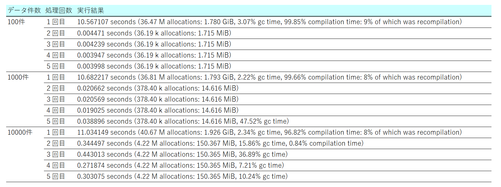
①について、1回目実行時のJIT (Just-In-Time) コンパイル時間の割合(X % completation time)が96~98%だったので、データ件数によりも JITコンパイルにかかった時間の割合 の影響が強く、差分がでなかった。
※Juliaは初回実行時、関数ごとに「引数の型」に応じてネイティブコードを生成(=JIT)する。この「ネイティブコードの生成にかかる時間」が compilation time としてカウントされ、JITコンパイル時間として表現されている。
②について、データ件数によってGarbage Collection(X % gc time)に差分が生じ、その影響によって処理時間の縮小度合いに差分が発生している。
※Garbage Collection:定期的に使われなくなったデータを検出し、メモリから削除(解放)しているもの
③について、Julia は JITコンパイルしたネイティブコードを「プロセスのメモリ上」にキャッシュしているため、2回目以降の処理時間が早くなる。
⇒PackageCompilerを使えば、立ち上げなおしても前回情報をもとに高速利用できるらしい。
参考資料
[1]svoboda, 『[Julia]VSCにおけるWSL2でのJulia 環境構築~サンプルコード実行まで』, https://qiita.com/svoboda/items/6a0ad624bc58a354edb3
[2]KristofferC, 『NearestNeighbors.jl』, https://github.com/KristofferC/NearestNeighbors.jl
[3]OkonSamuel ,『NearestNeighborModels.jl』,https://juliaai.github.io/NearestNeighborModels.jl/dev/
[4]plotly, 『kNN Classification in Juila』, https://plotly.com/julia/knn-classification/
[5]IanButterworth
,『PackageCompiler』,https://julialang.github.io/PackageCompiler.jl/dev/