[TF]Tensorboardを使って学習結果をVisualizationしてみた

Tensorboardを使って学習結果をVisualizationする方法を調べてみた。
Tensorboardに出力する方法はここを参考にした。

簡単な例

いきなり複雑なやつだと大変なので、簡単な例を作って試した。
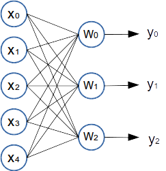
テストデータは下記の図のように、xは５次元、ｙを３次元とし、xをランダムで生成したあとに、あらかじめ指定しておいたWをかけてbを足してyを生成した。xが５次元、yが３次元なので、Wのサイズは5x3になる。
実行したコードは下記の通り、これはTensorflowのホームページのコードをテストデータに合わせてちょっとだけ変更した。

コードのポイントは下記の通り。
1. writer = tf.train.SummaryWriter("/tmp/tensorflow_log", sess.graph_def)のようにしてSummaryWriterのobjectを作る。そのときにlogを出力するdirectoryを指定する。
2. merged = tf.merge_all_summaries()でsummary dataを生成するoprationをまとめる。operationとはscalar_summaryとかhistogram_summaryのこと。
3. operationをコードに埋め込む。w_hist = tf.histogram_summary("weights", W)こんな感じ。
4. 何回かに１回（コードでは10回に1回）result = sess.run([merged, loss])のようにmergedを実行する。lossの方は、標準出力に出力するためなのでTensorboardに出したいだけであれば実行しなくてもいいと思う。
5. sess.runの戻り値をwriteに渡す。コードでは、mergedとlossをsess.runに渡しているのでresultがlistで戻ってくる。mergedの方なのでresult[0]をwriter.add_summary(summary_str, step)こんな感じで渡す。
6.学習を実行して終わったら、tensorboard --logdir=/tmp/tensorflow_log を実行する。
7.その状態でchromeを起動し、http://localhost:6006 にアクセスするとTensorBoardが表示され、logの出力がうまく行っているとGRAPHが表示される。

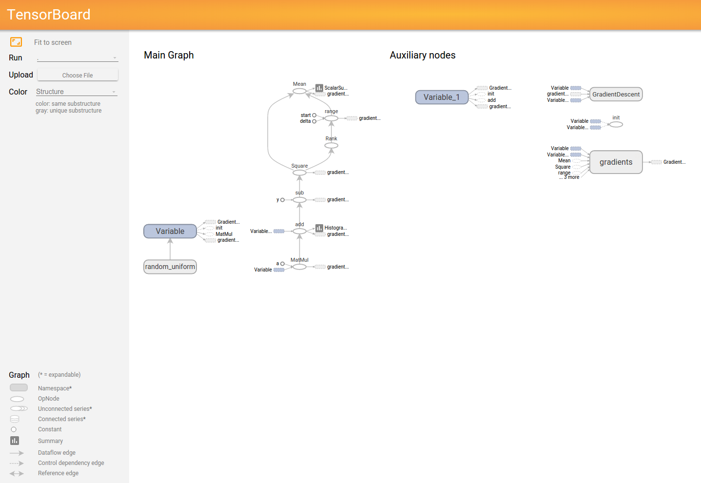
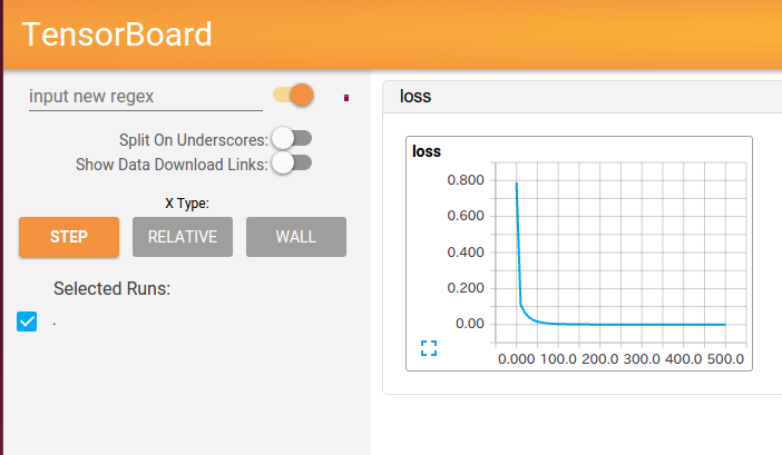
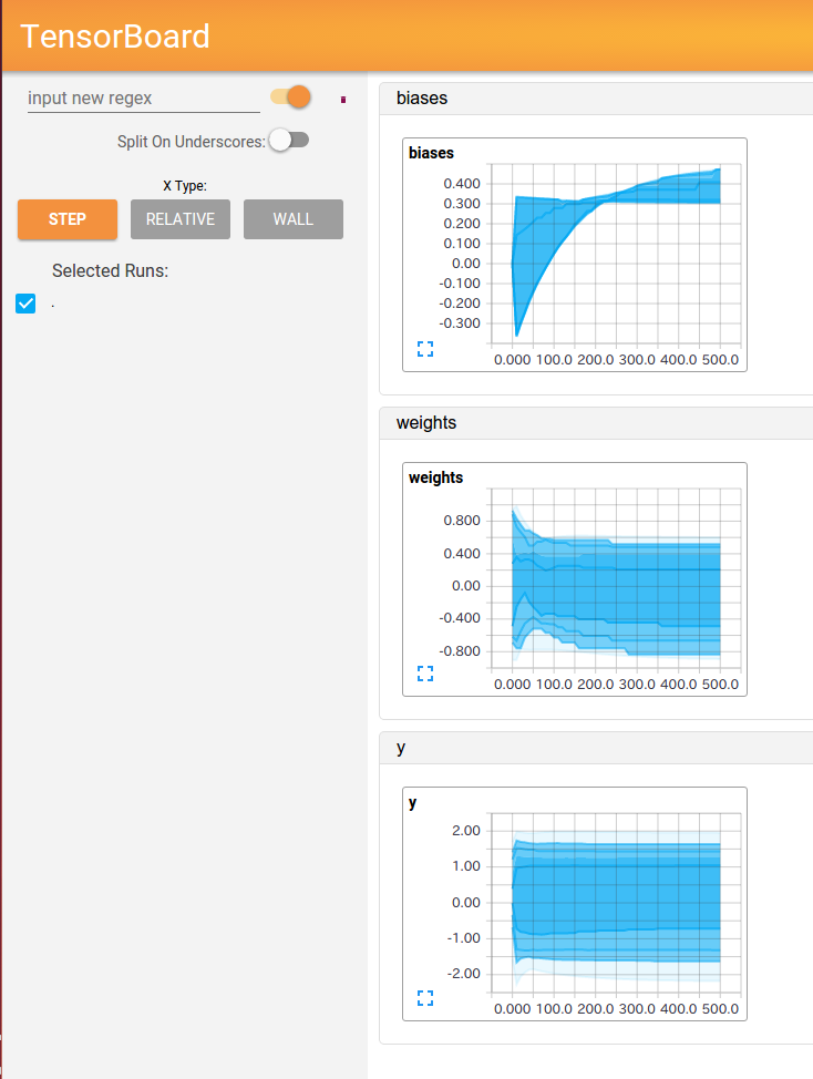
以下にTensorboardの結果と実行したコードを示す。

GRAPH

EVENTS

HISTOGRAMS

Code

python

import tensorflow as tf
import numpy as np

WW = np.array([[0.1, 0.6, -0.9], 
               [0.2, 0.5, -0.8], 
               [0.3, 0.4, -0.7],
               [0.4, 0.3, -0.6],
               [0.5, 0.2, -0.5]]).astype(np.float32)
bb = np.array([0.3, 0.4, 0.5]).astype(np.float32)
x_data = np.random.rand(100,5).astype(np.float32)
y_data = np.dot(x_data, WW) + bb

with tf.Session() as sess:

    W = tf.Variable(tf.random_uniform([5,3], -1.0, 1.0))
    # The zeros set to zero with all elements.
    b = tf.Variable(tf.zeros([3]))
    #y = W * x_data + b
    y = tf.matmul(x_data, W) + b

    # Add summary ops to collect data
    w_hist = tf.histogram_summary("weights", W)
    b_hist = tf.histogram_summary("biases", b)
    y_hist = tf.histogram_summary("y", y)

    # Minimize the mean squared errors.
    loss = tf.reduce_mean(tf.square(y - y_data))
    # Outputs a Summary protocol buffer with scalar values
    loss_summary = tf.scalar_summary("loss", loss)

    # Gradient descent algorithm
    optimizer = tf.train.GradientDescentOptimizer(0.5)
    train = optimizer.minimize(loss)

    # Before starting, initialize the variables.  We will 'run' this first.
    init = tf.initialize_all_variables()

    # Creates a SummaryWriter
    # Merges all summaries collected in the default graph
    merged = tf.merge_all_summaries()
    writer = tf.train.SummaryWriter("/tmp/tensorflow_log", sess.graph_def)
    sess.run(init)

    # Fit the line
    for step in xrange(501):
        if step % 10 == 0:
            result = sess.run([merged, loss])
            summary_str = result[0]
            acc = result[1]
            writer.add_summary(summary_str, step)
            print"step = %s acc = %s W = %s b = %s" % (step, acc, sess.run(W), sess.run(b))
        else:
            sess.run(train)

もうちょっと複雑な例

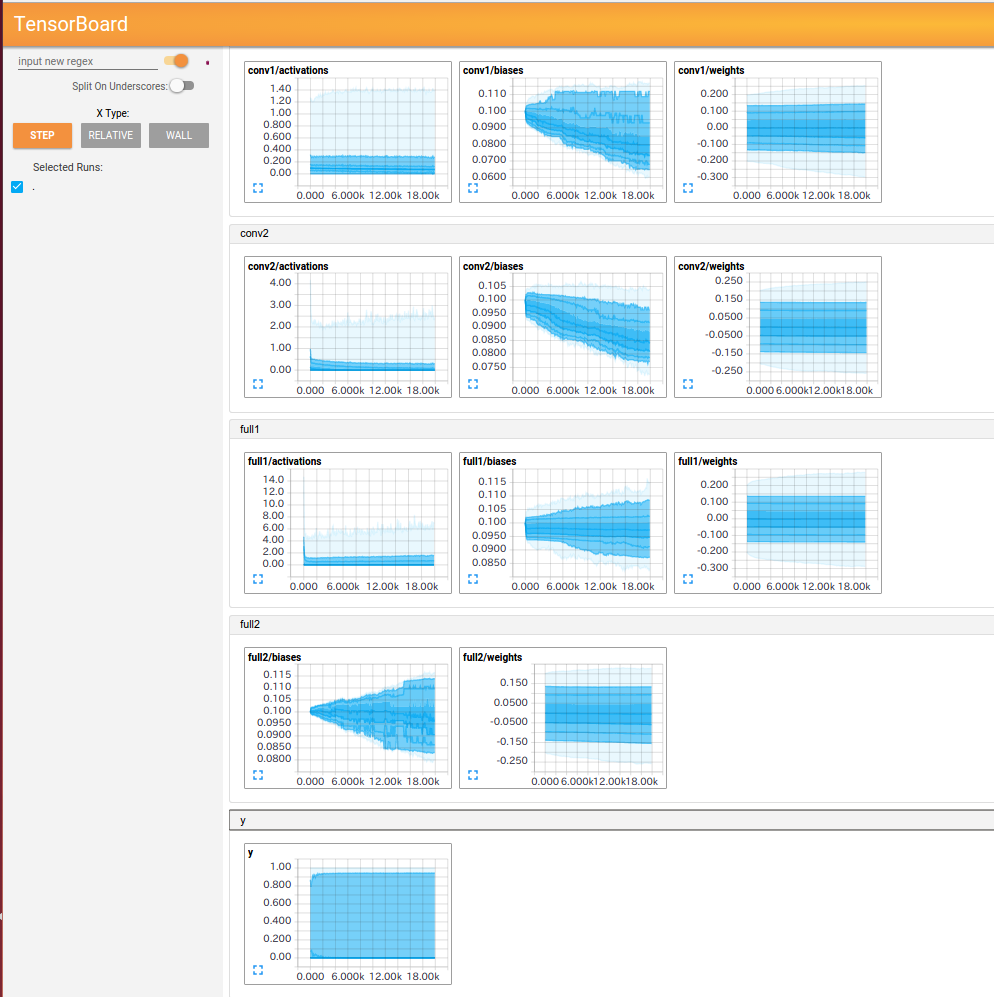
histogramをまとめるときは、tf.histogram_summary("xxx/weights", w), tf.histogram_summary("xxx/biases", b)のようにまとめたいhistogramのxxxを同じにする。
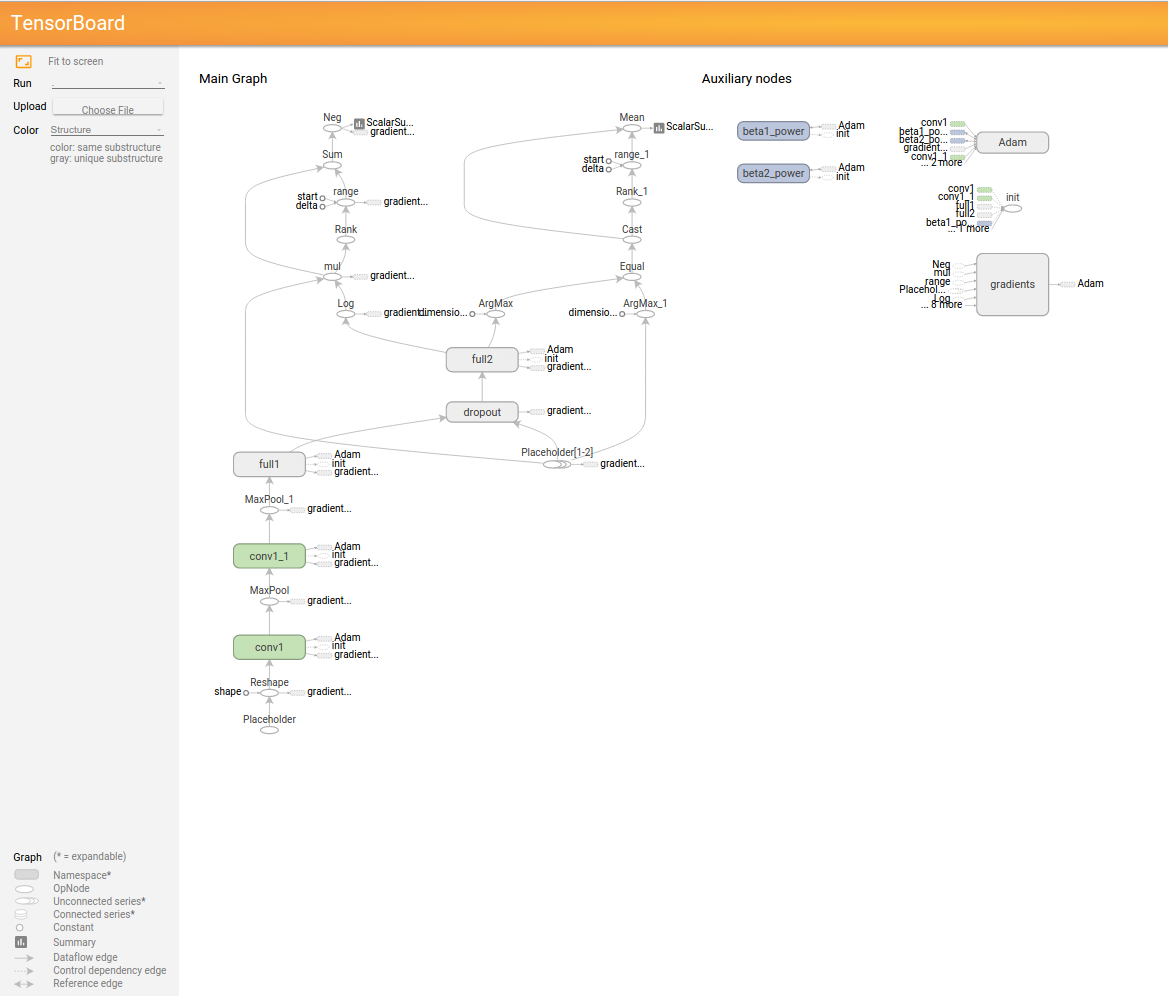
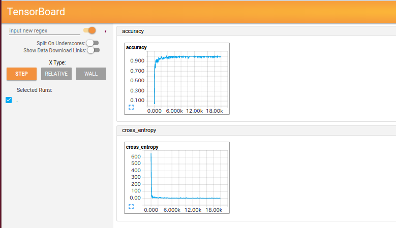
以下にTensorboardの結果と実行したコードを示す。

GRAPH

EVENTS

HISTOGRAMS

Code

python

import input_data
import tensorflow as tf

print 'load MNIST dataset'
mnist = input_data.read_data_sets("MNIST_data", one_hot=True)

def weight_variable(shape):
    initial = tf.truncated_normal(shape, stddev=0.1)
    return tf.Variable(initial)

def bias_variable(shape):
    initial = tf.constant(0.1, shape = shape)
    return tf.Variable(initial)

def conv2d(x, W):
    return tf.nn.conv2d(x, W, strides=[1,1,1,1], padding='SAME')
def max_pool_2x2(x):
    return tf.nn.max_pool(x, ksize=[1,2,2,1], strides=[1,2,2,1], padding='SAME')

def _write_histogram_summary(parent, infos):
    for i in infos:
        tf.histogram_summary("%s/%s" % (parent, i[0]), i[1])

with tf.Session() as sess:
    x = tf.placeholder("float", [None, 784])
    y_ = tf.placeholder("float", [None, 10])

    # 1x28x28 -> 32x28x28 -> 32x14x14
    x_image = tf.reshape(x, [-1,28,28,1])    
    with tf.variable_scope('conv1') as scope:
        W_conv1 = weight_variable([5, 5, 1, 32])
        b_conv1 = bias_variable([32])
        h_conv1 = tf.nn.relu(conv2d(x_image, W_conv1) + b_conv1, name=scope.name)

        _write_histogram_summary('conv1', [['weights', W_conv1],['biases', b_conv1], ['activations', h_conv1]])

    h_pool1 = max_pool_2x2(h_conv1)  

    # 32x14x14 -> 64x7x7
    with tf.variable_scope('conv1') as scope:
        W_conv2 = weight_variable([5, 5, 32, 64])
        b_conv2 = bias_variable([64])
        h_conv2 = tf.nn.relu(conv2d(h_pool1, W_conv2) + b_conv2, name=scope.name)

        _write_histogram_summary('conv2', [['weights', W_conv2],['biases', b_conv2], ['activations', h_conv2]])

    h_pool2 = max_pool_2x2(h_conv2)    

    # 64x7x7 -> 1024
    with tf.variable_scope('full1') as scope:
        W_fc1 = weight_variable([7 * 7 * 64, 1024])
        b_fc1 = bias_variable([1024])
        h_pool2_flat = tf.reshape(h_pool2, [-1, 7*7*64])
        h_fc1 = tf.nn.relu(tf.matmul(h_pool2_flat, W_fc1) + b_fc1, name=scope.name)    

        _write_histogram_summary('full1', [['weights', W_fc1],['biases', b_fc1], ['activations', h_fc1]])

    # dropout
    keep_prob = tf.placeholder("float")
    h_fc1_drop = tf.nn.dropout(h_fc1, keep_prob)

    # Readout
    with tf.variable_scope('full2') as scope:
        W_fc2 = weight_variable([1024, 10])
        b_fc2 = bias_variable([10])

        y_conv=tf.nn.softmax(tf.matmul(h_fc1_drop, W_fc2) + b_fc2, name=scope.name)  

        _write_histogram_summary('full2', [['weights', W_fc2],['biases', b_fc2]])

    tf.histogram_summary("y", y_conv)

    cross_entropy = -tf.reduce_sum(y_*tf.log(y_conv))

    train_step = tf.train.AdamOptimizer(1e-4).minimize(cross_entropy)
    correct_prediction = tf.equal(tf.argmax(y_conv,1), tf.argmax(y_,1))
    accuracy = tf.reduce_mean(tf.cast(correct_prediction, "float"))


    tf.scalar_summary("cross_entropy", cross_entropy)
    tf.scalar_summary("accuracy", accuracy)

    # Before starting, initialize the variables.  We will 'run' this first.
    init = tf.initialize_all_variables()

    # Creates a SummaryWriter
    # Merges all summaries collected in the default graph
    merged = tf.merge_all_summaries()
    writer = tf.train.SummaryWriter("/tmp/tensorflow_log_mnist", sess.graph_def)

    sess.run(init)

    # training
    N = len(mnist.train.images)
    N_test = len(mnist.test.images)
    n_epoch = 20000
    batchsize = 50

    for i in range(n_epoch):
        batch = mnist.train.next_batch(batchsize)
        if i%100 == 0:
            summary_str, loss_value = sess.run([merged, accuracy], feed_dict={x: batch[0], y_: batch[1], keep_prob: 0.5})
            writer.add_summary(summary_str, i)
            print "step %d %.2f" % (i, loss_value)
        sess.run(train_step, feed_dict={x: batch[0], y_: batch[1], keep_prob: 0.5})    

    tacc = 0
    tbatchsize = 1000
    for i in range(0,N_test,tbatchsize):
        acc = sess.run(accuracy, feed_dict={
        x: mnist.test.images[i:i+tbatchsize], y_: mnist.test.labels[i:i+tbatchsize], keep_prob: 1.0})
        tacc += acc * tbatchsize

        print "test step %d acc = %.2f" % (i//tbatchsize, acc)
    tacc /= N_test
    print "test accuracy %.2f" % tacc