コロナ第６波東京：簡易実行再生産数(Rt)を使ったピークアウト動的予測

初めに

全国的にコロナの第６波が襲来中ですが、コロナの波については、簡易実行再生産数(Rt)、勾配、新規陽性者数の中で、Rtが最も早くピークアウトすることが経験的に分かっています。Rtがピークアウトした後は、Rtの日次減衰率の値から、将来の新規養成者数のピーク日と最大新規陽性者数の予測値を計算することができます。この方法を用いて、東京のピークアウトを予測してみます。

簡易実行再生産数(Rt)とは

import os
import numpy as np
import pandas as pd
import random
import seaborn as sns
import datetime as datetime
import matplotlib.dates as dates
import matplotlib.pyplot as plt
import plotly.express as px
import plotly.graph_objects as go
from plotly.subplots import make_subplots

1. 使用データ

data0 = pd.read_csv("https://stopcovid19.metro.tokyo.lg.jp/data/130001_tokyo_covid19_patients.csv")
data0['date']=data0['公表_年月日']
data0['pcr_positives']=1
data1=data0[['date','pcr_positives']]
data1=data1.groupby('date',as_index=False).sum()
data1['positives mean 7-day']=data1['pcr_positives'].rolling(window=7).mean()
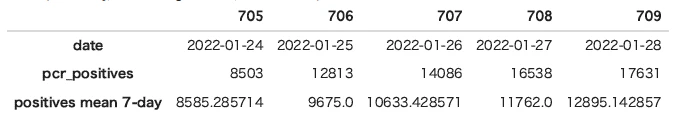
data1[-5:].T

2. 新規陽性者数

fig=make_subplots(specs=[[{"secondary_y":False}]])
fig.add_trace(go.Scatter(x=data1['date'][682:],y=data1['positives mean 7-day'][682:],name='positives mean 7-day'),secondary_y=False,)
fig.update_layout(autosize=False,width=500,height=300,title_text="Examined Positives (rolling 7-day) in Tokyo")
fig.update_xaxes(title_text="Date")
fig.update_yaxes(title_text="Cases",secondary_y=False)
fig.show()

3. 勾配(Slope)と簡易実効再生産数(Rt)の定義

簡易実効再生産数(Rt)の定義はこちらで紹介されているものと同じです。
https://www.niid.go.jp/niid/ja/diseases/ka/corona-virus/2019-ncov/2502-idsc/iasr-in/10465-496d04.html

col0=data1.columns.to_list()
col1=col0+['pm-7','slope']
data2=pd.DataFrame(columns=col1)
data2[col0]=data1
data2['pm-7']=data2['positives mean 7-day'].shift(7)
data2['slope']=(data2['positives mean 7-day']-data2['pm-7'])/7
data２['Rt']=data2['positives mean 7-day']/data2['pm-7']  
data3=data2[['date','pcr_positives','positives mean 7-day','slope','Rt']]
data4=data3[14:]

4. 日次減衰率と収束値の定義

from datetime import datetime
from datetime import date
from datetime import timedelta

# 最新データ日付、予測最終日の翌日
latest0 = datetime.strptime(data4['date'].max(),'%Y-%m-%d').date()
end0   = datetime.strptime('2022-05-01','%Y-%m-%d').date()

# 予測期間
dates0=[]
for i in range(1,(end0-latest0).days):
    dates0+=[(latest0+timedelta(i)).strftime('%Y-%m-%d') ]
print(dates0[0],dates0[-1])
# 2022-01-29 2022-04-30

# ７日前日付、最新データ日付
rt1_date=(latest0-timedelta(days=7)).strftime('%Y-%m-%d')
rt2_date=latest0.strftime('%Y-%m-%d')
print(rt1_date,rt2_date)
# 2022-01-21 2022-01-28
rt1=data4['Rt'][data4['date']==rt1_date].tolist()[0]
rt2=data4['Rt'][data4['date']==rt2_date].tolist()[0]
print(rt1,rt2)
# 3.1742696053305997 2.082212636386704

# 経験的に波が収束する時、Rt値はおよそ0.6位の値に収束します。 
# 最新のRtと7日前のRtから日次減衰率の平均値を計算します。
rt_conv=0.6 ### Rtの収束予想値
ratio=(rt2-rt_conv)/(rt1-rt_conv)
# factor**days=ratio
factor=10**(np.log10(ratio)/7)
print(factor) ### 日次減衰率
# 0.9241679987139932
# 波が収束するには日次減衰率<1.0であることが必要です。

# 予測期間前日までの実際のデータ
data5=data2[['date','positives mean 7-day', 'pm-7','slope','Rt']][682:].copy()

# 予測期間のデータ（計算前）
data5p=pd.DataFrame(columns=data5.columns)
data5p['date']=dates0
data5p.iloc[0:7,2]=data5.iloc[-7:,1]
data5p2=pd.concat([data5,data5p],axis=0).reset_index(drop=True)
length0=len(data5) #既存データ日数
length2=len(data5p2) #全期間日数（既存データ日数＋予測期間日数）

5. 予測値の計算

# 予測期間のデータの計算
for j in range(16):
    for i in range(length0,length2):
        data5p2.loc[i,'Rt']=(data5p2.loc[i-1,'Rt']-rt_conv)*factor+rt_conv
        data5p2.loc[i,'positives mean 7-day']=data5p2.loc[i,'pm-7']*data5p2.loc[i,'Rt']
        data5p2['slope']=(data5p2['positives mean 7-day']-data5p2['pm-7'])/7
        data5p2.loc[i+7,'pm-7']=data5p2.loc[i,'positives mean 7-day']

# 全期間のデータ（計算後）
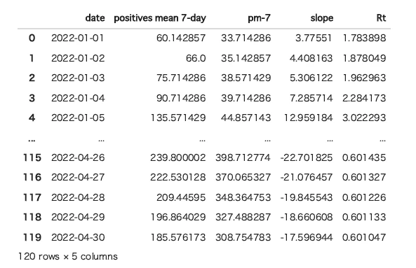
data5p2[:length2]

6. 計算結果

# 最新の予測結果の出力
pred_date=latest0
decay_rate=factor
slope_max_date=data5p2['date'][data5p2['slope']==data5p2['slope'].max()].tolist()[0]
slope_max_num=data5p2['slope'][data5p2['slope']==data5p2['slope'].max()].tolist()[0]
posi_max_date=data5p2['date'][data5p2['positives mean 7-day']==data5p2['positives mean 7-day'].max()].tolist()[0]
posi_max_num=data5p2['positives mean 7-day'][data5p2['positives mean 7-day']==data5p2['positives mean 7-day'].max()].tolist()[0]

print('Decay_Rate',round(decay_rate,4),'on',pred_date,', Slope_Max',round(slope_max_num),'on',slope_max_date,', Positives_Max',round(posi_max_num),'on',posi_max_date)
# Decay_Rate 0.9242 on 2022-01-28 , Slope_Max 990 on 2022-01-29 , Positives_Max 20604 on 2022-02-12

fig=make_subplots(specs=[[{"secondary_y":False}]])
fig.add_trace(go.Scatter(x=data5p2['date'][0:length0],y=data5p2['Rt'][0:length0],name='actual'),secondary_y=False,)
fig.add_trace(go.Scatter(x=data5p2['date'][length0-1:],y=data5p2['Rt'][length0-1:],name='predicted'),secondary_y=False,)
fig.update_layout(autosize=False,width=500,height=300,title_text="Rt change in Tokyo")
fig.update_xaxes(title_text="Date")
fig.update_yaxes(title_text="Rt",secondary_y=False)
fig.show()

fig=make_subplots(specs=[[{"secondary_y":False}]])
fig.add_trace(go.Scatter(x=data5p2['date'][0:length0],y=data5p2['slope'][0:length0],name='actual'),secondary_y=False,)
fig.add_trace(go.Scatter(x=data5p2['date'][length0-1:],y=data5p2['slope'][length0-1:],name='predicted'),secondary_y=False,)
fig.update_layout(autosize=False,width=500,height=300,title_text="Slope change in Tokyo")
fig.update_xaxes(title_text="Date")
fig.update_yaxes(title_text="Slope",secondary_y=False)
fig.show()

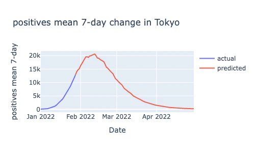
fig=make_subplots(specs=[[{"secondary_y":False}]])
fig.add_trace(go.Scatter(x=data5p2['date'][0:length0],y=data5p2['positives mean 7-day'][0:length0],name='actual'),secondary_y=False,)
fig.add_trace(go.Scatter(x=data5p2['date'][length0-1:],y=data5p2['positives mean 7-day'][length0-1:],name='predicted'),secondary_y=False,)
fig.update_layout(autosize=False,width=500,height=300,title_text="positives mean 7-day change in Tokyo")
fig.update_xaxes(title_text="Date")
fig.update_yaxes(title_text="positives mean 7-day",secondary_y=False)
fig.show()

終わりに

以下のページでピークアウトの予測履歴を確認できます。
https://www.kaggle.com/stpeteishii/covid19-tokyo-6th-wave-future-prediction