前置き
本記事は、日本語CLIPモデルに関するシリーズ記事の2本目です。
日本語CLIPモデルとは何なのかについては、1本目の記事「【日本語モデル付き】2022年にマルチモーダル処理をする人にお勧めしたい事前学習済みモデル」をご覧ください。
本記事では、日本語CLIPモデルを用いて次の3つの基本的処理を行う方法について説明します。
- 画像とテキストの類似度計算(日本語CLIPモデルの傾向分析も)
- 画像やテキストの埋め込みベクトル計算
- 画像やテキストによる類似画像検索
本記事を読めば、例えば、下図のような画像とテキスト(説明文)の間の類似度計算や類似検索が行えるようになります。
画像:
類似度(Y軸は画像、X軸はテキスト):

本記事の内容は次のColaboratory Notebookを実行すれば再現可能です。改造も容易でしょう。
- Colabで直接開く: https://colab.research.google.com/github/sonoisa/clip-japanese/blob/main/CLIP_ja_basics.ipynb
- Githubで開く: https://github.com/sonoisa/clip-japanese/blob/main/CLIP_ja_basics.ipynb
準備
準備として、依存ライブラリのインストールやサンプル画像のダウンロード、各種クラスの定義を行います。
ライブラリとサンプル画像の準備
transformers/fugashi/ipadicは日本語CLIPの利用に必要なライブラリで、japanize-matplotlibはこのサンプルコード用の、matplotlibで日本語を表示するためのライブラリです。
%%capture
!pip install transformers==4.14.0 fugashi ipadic
!pip install japanize-matplotlib
このサンプルコードでは https://github.com/sonoisa/clip-japanese/tree/main/sample_images に用意した16枚の画像を利用します。
!git clone https://github.com/sonoisa/clip-japanese
日本語CLIPクラス
日本語CLIPモデルを表すクラスを定義します。クラスは次の3つで構成されます。
- ClipTextModel: CLIPのテキストエンコーダーモデル
- ClipVisionModel: CLIPの画像エンコーダーモデル
- ClipModel: CLIPモデル。ClipTextModelとClipVisionModelの両方を内包する。
どのクラスも基本構造は同じで、学習済みモデルの読み込み(__init__)、テキストや画像のエンコード(encode*)、推論(forward)、保存(save)を行うメソッドを持っています。
その中でも特に重要なのがエンコードメソッド(encode_text/encode_image/encode)です。
本記事ではエンコードメソッドの使いこなし方について例を用いて説明をしていきます。
import os
import torch
from torch import nn
from transformers import AutoModel, AutoTokenizer
from huggingface_hub import hf_hub_download


class ClipTextModel(nn.Module):
    def __init__(self, model_name_or_path, device=None):
        super(ClipTextModel, self).__init__()

        if os.path.exists(model_name_or_path):
            # load from file system
            output_linear_state_dict = torch.load(os.path.join(model_name_or_path, "output_linear.bin"), map_location=device)
        else:
            # download from the Hugging Face model hub
            filename = hf_hub_download(repo_id=model_name_or_path, filename="output_linear.bin")
            output_linear_state_dict = torch.load(filename)

        self.model = AutoModel.from_pretrained(model_name_or_path)
        config = self.model.config

        self.max_cls_depth = 6

        sentence_vector_size = output_linear_state_dict["bias"].shape[0]
        self.sentence_vector_size = sentence_vector_size
        self.output_linear = nn.Linear(self.max_cls_depth * config.hidden_size, sentence_vector_size)
        self.output_linear.load_state_dict(output_linear_state_dict)

        self.tokenizer = AutoTokenizer.from_pretrained(model_name_or_path,
                                                       is_fast=True, do_lower_case=True)

        self.eval()

        if device is None:
            device = "cuda" if torch.cuda.is_available() else "cpu"
        self.device = torch.device(device)
        self.to(self.device)

    def forward(
        self,
        input_ids=None,
        attention_mask=None,
        token_type_ids=None,
    ):
        output_states = self.model(
            input_ids,
            attention_mask=attention_mask,
            token_type_ids=token_type_ids,
            position_ids=None,
            head_mask=None,
            inputs_embeds=None,
            output_attentions=None,
            output_hidden_states=True,
            return_dict=True,
        )
        token_embeddings = output_states[0]
        input_mask_expanded = attention_mask.unsqueeze(-1).expand(token_embeddings.size()).float()
        hidden_states = output_states["hidden_states"]

        output_vectors = []

        # cls tokens
        for i in range(1, self.max_cls_depth + 1):
            cls_token = hidden_states[-1 * i][:, 0]
            output_vectors.append(cls_token)

        output_vector = torch.cat(output_vectors, dim=1)
        logits = self.output_linear(output_vector)

        output = (logits,) + output_states[2:]
        return output

    @torch.no_grad()
    def encode_text(self, texts, batch_size=8, max_length=64):
        model.eval()
        all_embeddings = []
        iterator = range(0, len(texts), batch_size)
        for batch_idx in iterator:
            batch = texts[batch_idx:batch_idx + batch_size]

            encoded_input = self.tokenizer.batch_encode_plus(
                batch, max_length=max_length, padding="longest",
                truncation=True, return_tensors="pt").to(self.device)
            model_output = self(**encoded_input)
            text_embeddings = model_output[0].cpu()

            all_embeddings.extend(text_embeddings)

        # return torch.stack(all_embeddings).numpy()
        return torch.stack(all_embeddings)

    def save(self, output_dir):
        self.model.save_pretrained(output_dir)
        self.tokenizer.save_pretrained(output_dir)
        torch.save(self.output_linear.state_dict(), os.path.join(output_dir, "output_linear.bin"))
import os
import torch
from torch import nn
import transformers
from huggingface_hub import hf_hub_download


class ClipVisionModel(nn.Module):
    def __init__(self, model_name_or_path, device=None):
        super(ClipVisionModel, self).__init__()

        if os.path.exists(model_name_or_path):
            # load from file system
            visual_projection_state_dict = torch.load(os.path.join(model_name_or_path, "visual_projection.bin"))
        else:
            # download from the Hugging Face model hub
            filename = hf_hub_download(repo_id=model_name_or_path, filename="visual_projection.bin")
            visual_projection_state_dict = torch.load(filename)

        self.model = transformers.CLIPVisionModel.from_pretrained(model_name_or_path)
        config = self.model.config

        self.feature_extractor = transformers.CLIPFeatureExtractor.from_pretrained(model_name_or_path)

        vision_embed_dim = config.hidden_size
        projection_dim = 512

        self.visual_projection = nn.Linear(vision_embed_dim, projection_dim, bias=False)
        self.visual_projection.load_state_dict(visual_projection_state_dict)

        self.eval()

        if device is None:
            device = "cuda" if torch.cuda.is_available() else "cpu"
        self.device = torch.device(device)
        self.to(self.device)

    def forward(
        self,
        pixel_values=None,
        output_attentions=None,
        output_hidden_states=None,
        return_dict=None,
    ):
        output_states = self.model(
            pixel_values=pixel_values,
            output_attentions=output_attentions,
            output_hidden_states=output_hidden_states,
            return_dict=return_dict,
        )
        image_embeds = self.visual_projection(output_states[1])

        return image_embeds

    @torch.no_grad()
    def encode_image(self, images, batch_size=8):
        model.eval()
        all_embeddings = []
        iterator = range(0, len(images), batch_size)
        for batch_idx in iterator:
            batch = images[batch_idx:batch_idx + batch_size]

            encoded_input = self.feature_extractor(batch, return_tensors="pt").to(self.device)
            model_output = self(**encoded_input)
            image_embeddings = model_output.cpu()

            all_embeddings.extend(image_embeddings)

        # return torch.stack(all_embeddings).numpy()
        return torch.stack(all_embeddings)

    @staticmethod
    def remove_alpha_channel(image):
        image.convert("RGBA")
        alpha = image.convert('RGBA').split()[-1]
        background = Image.new("RGBA", image.size, (255, 255, 255))
        background.paste(image, mask=alpha)
        image = background.convert("RGB")
        return image

    def save(self, output_dir):
        self.model.save_pretrained(output_dir)
        self.feature_extractor.save_pretrained(output_dir)
        torch.save(self.visual_projection.state_dict(), os.path.join(output_dir, "visual_projection.bin"))
import os
import torch
from torch import nn
from huggingface_hub import snapshot_download


class ClipModel(nn.Module):
    def __init__(self, model_name_or_path, device=None):
        super(ClipModel, self).__init__()

        if os.path.exists(model_name_or_path):
            # load from file system
            repo_dir = model_name_or_path
        else:
            # download from the Hugging Face model hub
            repo_dir = snapshot_download(model_name_or_path)

        self.text_model = ClipTextModel(repo_dir, device=device)
        self.vision_model = ClipVisionModel(os.path.join(repo_dir, "vision_model"), device=device)

        with torch.no_grad():
            logit_scale = nn.Parameter(torch.ones([]) * 2.6592)
            logit_scale.set_(torch.load(os.path.join(repo_dir, "logit_scale.bin"), map_location=device).clone().cpu())
            self.logit_scale = logit_scale

        self.eval()

        if device is None:
            device = "cuda" if torch.cuda.is_available() else "cpu"
        self.device = torch.device(device)
        self.to(self.device)

    def forward(self, pixel_values, input_ids, attention_mask, token_type_ids):
        image_features = self.vision_model(pixel_values=pixel_values)
        text_features = self.text_model(input_ids=input_ids,
                                        attention_mask=attention_mask,
                                        token_type_ids=token_type_ids)[0]

        image_features = image_features / image_features.norm(dim=-1, keepdim=True)
        text_features = text_features / text_features.norm(dim=-1, keepdim=True)

        logit_scale = self.logit_scale.exp()
        logits_per_image = logit_scale * image_features @ text_features.t()
        logits_per_text = logits_per_image.t()

        return logits_per_image, logits_per_text

    @torch.no_grad()
    def encode(self, images, texts, batch_size=8, max_length=64):
        model.eval()
        image_features = self.vision_model.encode_image(images, batch_size=batch_size)
        text_features = self.text_model.encode_text(texts, batch_size=batch_size, max_length=max_length)

        image_features = image_features.to(self.device)
        text_features = text_features.to(self.device)

        image_features = image_features / image_features.norm(dim=-1, keepdim=True)
        text_features = text_features / text_features.norm(dim=-1, keepdim=True)

        logit_scale = self.logit_scale.exp()
        logits_per_image = logit_scale * image_features @ text_features.t()
        logits_per_text = logits_per_image.t()

        logits_per_image = logits_per_image.cpu()
        logits_per_text = logits_per_text.cpu()

        return logits_per_image, logits_per_text

    def save(self, output_dir):
        torch.save(self.logit_scale, os.path.join(output_dir, "logit_scale.bin"))
        self.text_model.save(output_dir)
        self.vision_model.save(os.path.join(output_dir, "vision_model"))
テキストの正規化処理定義
テキストの正規化処理を定義します。
これは https://github.com/neologd/mecab-ipadic-neologd/wiki/Regexp.ja の正規化処理のうち、チルダを残すように微変更したものです。
日本語CLIPを用いてテキストをエンコードする場合はこの正規化処理を行う必要があります。もし、行わないと精度が落ちる可能性があります。
# https://github.com/neologd/mecab-ipadic-neologd/wiki/Regexp.ja から引用・一部改変
from __future__ import unicode_literals
import re
import unicodedata

def unicode_normalize(cls, s):
    pt = re.compile('([{}]+)'.format(cls))

    def norm(c):
        return unicodedata.normalize('NFKC', c) if pt.match(c) else c

    s = ''.join(norm(x) for x in re.split(pt, s))
    s = re.sub('-', '-', s)
    return s

def remove_extra_spaces(s):
    s = re.sub('[  ]+', ' ', s)
    blocks = ''.join(('\u4E00-\u9FFF',  # CJK UNIFIED IDEOGRAPHS
                      '\u3040-\u309F',  # HIRAGANA
                      '\u30A0-\u30FF',  # KATAKANA
                      '\u3000-\u303F',  # CJK SYMBOLS AND PUNCTUATION
                      '\uFF00-\uFFEF'   # HALFWIDTH AND FULLWIDTH FORMS
                      ))
    basic_latin = '\u0000-\u007F'

    def remove_space_between(cls1, cls2, s):
        p = re.compile('([{}]) ([{}])'.format(cls1, cls2))
        while p.search(s):
            s = p.sub(r'\1\2', s)
        return s

    s = remove_space_between(blocks, blocks, s)
    s = remove_space_between(blocks, basic_latin, s)
    s = remove_space_between(basic_latin, blocks, s)
    return s

def normalize_neologd(s):
    s = s.strip()
    s = unicode_normalize('0-9A-Za-z。-゚', s)

    def maketrans(f, t):
        return {ord(x): ord(y) for x, y in zip(f, t)}

    s = re.sub('[˗֊‐‑‒–⁃⁻₋−]+', '-', s)  # normalize hyphens
    s = re.sub('[﹣-ー—―─━ー]+', 'ー', s)  # normalize choonpus
    s = re.sub('[~∼∾〜〰~]+', '〜', s)  # normalize tildes (modified by Isao Sonobe)
    s = s.translate(
        maketrans('!"#$%&\'()*+,-./:;<=>?@[¥]^_`{|}~。、・「」',
              '!”#$%&’()*+,-./:;<=>?@[¥]^_`{|}〜。、・「」'))

    s = remove_extra_spaces(s)
    s = unicode_normalize('!”#$%&’()*+,-./:;<>?@[¥]^_`{|}〜', s)  # keep =,・,「,」
    s = re.sub('[’]', '\'', s)
    s = re.sub('[”]', '"', s)
    s = s.lower()
    return s

def normalize_text(text):
    return normalize_neologd(text)
学習済み日本語CLIPモデルのダウンロード
次のコードを実行してHugging Face Model Hubで公開している学習済み日本語CLIPモデルをダウンロードします。
import torch

device = "cuda" if torch.cuda.is_available() else "cpu"
model = ClipModel("sonoisa/clip-vit-b-32-japanese-v1", device=device)
これで日本語CLIPモデルを利用する準備が完了しました。
続いて日本語CLIPの典型的な応用方法を3つ説明します。
1. 画像とテキストの類似度計算
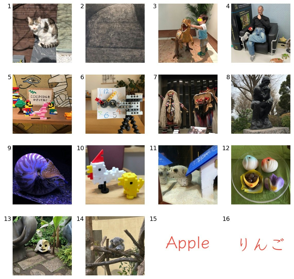
このセクションでは、16枚の画像について文章との類似度を求める方法について説明します。
画像の確認
まずは次のコードを実行して16枚のサンプル画像を見てみましょう。
import matplotlib.pyplot as plt
from PIL import Image

# 類似度を求める対象の画像(16枚)
images = [Image.open(f"/content/clip-japanese/sample_images/{i}.jpeg") for i in range(1, 17)]

# タイリング表示
plt.figure(dpi=140, figsize=(10,10))

for i in range(len(images)):
    sp = plt.subplot(4, 4, i + 1)
    plt.imshow(images[i])
    text = sp.text(-16, 0, f"{i + 1}", ha="right", va="top", color="black", fontsize=12)
    plt.axis("off")
Out[8]
説明不要のものもあるでしょうが、被写体は次の通りです。
- 猫
- ロゼッタストーン(国立民族学博物館)
- 恐竜の模型と子供(国立科学博物館)
- ジョブズ人形(どこから入手したか失念)
- レゴでできたマリオとルイージ?(レゴランド・ジャパン、見知らぬ誰かの作品)
- レゴでできた時計
- 魔女ランダと聖獣バロン(国立民族学博物館)
- 彫刻「考える人」(国立西洋美術館)
- アンモナイト(八景島アクアミュージアム)
- ニューブロックで作った鶏とヒヨコ
- コクテンフグ(ヨコハマおもしろ水族館)
- こどもの日をテーマにした和菓子
- 彫刻「午後の日」(岡本太郎記念館)
- 眠っているコアラ(多摩動物公園)
- Apple
- りんご
画像とテキストの類似度計算
それでは画像とテキストの類似度を計算します。
画像との類似度を計算するテキストは次のコードのtextsです。コードのコメントに確認したいことが書かれています。
画像とテキストの類似度計算は、画像とテキストを引数にmodel.encode()を呼び出し、戻り値にsoftmaxを適用するだけです。model.encode()の戻り値の意味は次のとおりです。
- logits_per_imageのsoftmaxをとると、1つの画像に関する各文章の類似度(合計1.0)になります。
- logits_per_textのsoftmaxをとると、1つの文章に関する各画像の類似度(合計1.0)になります。
このサンプルコードでは、各画像について、テキストとの類似性を計算することにします(従って、logits_per_imageを利用しています)。
import torch

# 画像との類似度を求める文章
texts = ["猫",
         "ロゼッタストーン",
         "恐竜と子供", "恐竜", "子供",  # 複数の物体が写っているとき、全体を見て類似性を判定するか?
         "考えるスティーブ・ジョブズの人形",  # 考える人との混同が起きないか?
         "レゴでできたマリオやルイージなど",  # レゴやマリオといった固有名詞を認識できるか?
         "レゴでできた時計",  # 時計に見えるかギリギリのものを認識できるか?
         "魔女ランダと聖獣バロン", "特殊合体するとシヴァ神",  # あまりメジャーではなさそうな存在を認識できるか?
         "彫刻「考える人」",  # 考えるスティーブ・ジョブズとの混同が起きないか?
         "水槽の中のアンモナイト",  # コクテンフグと見分けがつくか?
         "鶏とヒヨコのおもちゃ",  # 抽象的な造形表現を認識できるか?
         "水槽の中の犬", "水槽の中のコクテンフグ",  # 犬と錯覚するか?
         "お菓子が1個", "お菓子が2個", "お菓子が3個", "お菓子が4個", "お菓子が5個",  # 数勘定できるか?
         "彫刻「午後の日」", "芸術作品",  # 日本の芸術作品を認識できるか?
         "眠るコアラ", "木登りするコアラ",  # 行動を識別できるか?
         "Apple", "Pineapple",  # アルファベットを認識できるか?(英語版CLIPではできるため、できなくなっていないかの確認)
         "りんご", "パイナップル",  # ひらがなを認識できるか?
        ]

texts = [normalize_text(text) for text in texts]  # この正規化は必須です。行わないと精度が落ちることがあります。

logits_per_image, logits_per_text = model.encode(images, texts)

similarity_per_image = torch.softmax(logits_per_image, dim=1)
類似度の可視化
画像と文章との類似度を可視化します。
https://stackoverflow.com/questions/8897593/how-to-compute-the-similarity-between-two-text-documents を参考にしました。
# ref. https://stackoverflow.com/questions/8897593/how-to-compute-the-similarity-between-two-text-documents
import matplotlib.pyplot as plt
import matplotlib.patches as patches
import japanize_matplotlib
import numpy as np

def heatmap(x_labels, y_labels, expected_answers, values):
    fig, ax = plt.subplots(dpi=140, figsize=(8, 8))
    im = ax.imshow(values, vmin=0, vmax=1, cmap="viridis")

    ax.set_xticks(np.arange(len(x_labels)))
    ax.set_yticks(np.arange(len(y_labels)))
    ax.set_xticklabels(x_labels)
    ax.set_yticklabels(y_labels)
    ax.set_xlabel("テキスト")
    ax.set_ylabel("画像")

    plt.setp(ax.get_xticklabels(), rotation=60, ha="right", fontsize=10,
            rotation_mode="anchor")

    for i in range(len(y_labels)):
        for j in range(len(x_labels)):
            ax.text(j, i, "%.2f" % values[i, j],
                    ha="center", va="center", color="w", fontsize=6)
            if expected_answers[i] == j:
                c = patches.Circle(xy=(j, i), radius=0.5, ec='r', fill=False)
                ax.add_patch(c)

    fig.tight_layout()
    plt.show()

x_labels = texts
y_labels = ["1. 猫", "2. ロゼッタストーン", "3. 恐竜と子供", "4. ジョブズの人形",
            "5. レゴでできたマリオなど", "6. レゴでできた時計", "7. 魔女ランダと聖獣バロン",
            "8. 彫刻「考える人」", "9. アンモナイト", "10. 鶏とヒヨコのおもちゃ", "11. コクテンフグ",
            "12. 和菓子", "13. 彫刻「午後の日」", "14. コアラ", "15. Apple",
            "16. りんご"]
expected_answers = [0, 1, 2, 5, 6, 7, 8, 10, 11, 12, 14, 18, 20, 22, 24, 26]
heatmap(x_labels, y_labels, expected_answers, similarity_per_image)
可視化結果は下図のようになります。
画像(Y軸)ごとに、その画像と各テキスト(X軸)の類似度を示します。
赤丸は想定した答えを表しています。彫刻「午後の日」と「りんご」以外は正解していますね。
Out[10]
結果分析
日本語CLIPモデルを用いた、画像とテキストの類似度計算結果からその挙動の傾向を分析してみます。
まずは分析のサマリからです。
- 画像に写っている物体とテキストの単語の一個一個の近さではなく、画像とテキストが総合的に表している意味の近さで、類似性が評価される。構成要素の組み合わせによって生まれる総合的意味や、抽象的な造形表現、物が行なっている動作など。
- 固有名詞(固有な物体)も問題なく認識できているが、BERTの事前学習において出現頻度が低かったであろうカタカナ固有名詞(例:ランダやバロン、シヴァ、コクテンフグ、岡本太郎の「午後の日」)は苦手な傾向がありそうである。
- 個数を数えることができる。ただし、±1の範囲内で。
- 画像中の英語文字を認識できる。日本語文字は認識できない。
もちろん少数サンプルでの評価結果でしかありませんので、一般論にするにはより大規模な分析が必要です。
以下、詳細です。
画像ごとに分析をしていきますので、大変お手数ですがOut[10]の図を別ウィンドウに開いて参照しながら以下の分析をお読みください。
1.猫

これは簡単すぎる問題だったようです。少しは「コアラ」というテキストとも近くなるかと思いましたが類似度は0.00でした。
2.ロゼッタストーン

ちょっと分かりにくい画像ですが正解しています。テキスト「芸術作品」に0.11ほど出ているのも納得感あります。
3.恐竜と子供

これは複数の物体が写っているとき、全体を見て類似性を判定できるかテストしてみた例でした。
ちゃんとテキスト「恐竜と子供」との類似度が0.99と非常に高くなっています。
少しは単独の「恐竜」や「子供」とも迷うかなと思っていましたが、迷わず判定できているのはすごいです。
4.ジョブズの人形

テキストに「考える」を入れることで「考える人」との混同が起きないかのテストです。
特に混同が発生することなく両者を見分けられています。どちらも有名人(?)ですが。
単語ひとつひとつではなく、テキスト全体の意味をエンコードするモデルになっているからと思われます。
5.レゴでできたマリオなど

これはレゴやマリオといった固有名詞を認識できるか試してみるテストです。
結果は「レゴでできたマリオやルイージなど」と「レゴでできた時計」で多少迷っています。
レゴでできたマリオの画像にはマリオ以外にも色々な目立つ物体が写っていることが迷いが生じた原因かもしれません。
6.レゴでできた時計

あまり分かりやすい時計の形状ではないが、長針や短針、1から12までの数字といった時計の構成要素を持つものを総合して時計と認識できるかテストしたものです。
結果、簡単な問題だったようです。
7.魔女ランダと聖獣バロン

あまりメジャーではなさそうな「魔女ランダと聖獣バロン」を認識できるかテストしたものです。
これは悩んでいるようでテキスト「魔女ランダと聖獣バロン」との類似度は0.61と低く、テキスト「特殊合体するとシヴァ神」と0.11、「芸術作品」と0.07、「お菓子が2個」と0.04など、迷っているのが見えます。
「特殊合体するとシヴァ神」はボケ(参考:シヴァ(女神転生))として入れたものなので2位に出てくると逆に戸惑ってしまいますが、同じ宗教儀式的(同じヒンドゥー教的)な何かを特徴量として捉えられていると言えそうです。
また、「お菓子が2個」に反応しているのは2体であることがエンコードされているからでしょう。
8.彫刻「考える人」

これはテキスト「考えるスティーブ・ジョブズの人形」との混同が起きないかテストしたものですが全く問題ないですね。
9.アンモナイト

これは簡単な問題かと思っていましたが、意外なことに少し迷っているようです。
テキスト「水槽の中のコクテンフグ」にも0.13ほど類似していると判定しています。
水生生物までは絞り込めているけれども、その先で迷いが出ています。
これは後述するコクテンフグでも同様です。
10.鶏とヒヨコのおもちゃ

Gakkenニューブロックで作った鶏とヒヨコです。
レゴでできた時計に続き、抽象的な造形物を認識できるかのテストでしたが、簡単だったようです。
11.コクテンフグ

顔が犬そっくりであることで有名なフグです。
また紛らわしいことに横に犬小屋も写っているという念の入れようです。
犬に錯覚しないかテストしてみました。結果としては正解。
関心のあったテキスト「水槽の中の犬」との類似度は0.08でした。その気持ち分かります。
意外なことに「水槽の中のアンモナイト」には0.26大きく類似していると判定しています。
水生生物であることまでは認識できているけれども、その名前はあまり自信がないようです。
事前学習において出現頻度の低いカタカナ固有名詞は苦手である可能性もあります。
12.和菓子

これは数をカウントできるかのテストです。
僅差ですが、テキスト「お菓子が4個」に最も類似し、その前後の個数のものにも次に類似するという傾向が出ています。
個数の情報も捉えられているようです。
13.彫刻「午後の日」

岡本太郎の作品「午後の日」です。
これは日本の芸術作品を認識できるかという実験です。
結果としては不正解でした。
画像と大きく類似するテキストはないという結果になっています。
14.コアラ

コアラであることに認識は簡単だとして、動作を識別できるかテストしてみました。
正解であるテキスト「眠るコアラ」との類似度は0.93、不正解であるが登場する物体は重なる「木登りするコアラ」は0.07と、物体だけでなく、その動作の種類も正しく識別できることが分かりました。これは応用上嬉しい性質です。
15.Apple

英語版CLIPではOCRという程ではないものの文字を認識できることが知られており、その性質が失われていないかテストする例です。
テキスト「apple」に0.75、「りんご」に0.25だけ類似しているという結果になりました。
一部文字が重なる「pineapple」には全く類似しない(類似度 0.00)と正しく判定されています。
16.りんご

日本語の文字も認識できるか実験です。
とはいえ、OpenAIが英語版CLIPを作成したときの学習データには日本語テキストは入っていないので、無理だろうことは承知で行ったテストです。
結果は不正解です(ま、そうですよね)。
画像と大きく類似するテキストはないという結果になっています。
つまり、画像内に文字情報も現れるタスクに対してCLIPを応用(転移学習や特徴量生成など)する場合、その文字情報が英語なのか、日本語なのかで大きく精度が変わりうることが予想されます(要実験)。
2. 画像とテキストの埋め込みベクトル計算
画像とテキストの埋め込みベクトルを得る方法について説明します。
埋め込みベクトルの主な用途としては、類似画像検索や、画像やテキストの特徴量計算があるでしょう。
まずは画像の埋め込みベクトルを計算します。
model.vision_modelのencode_image(images)を呼び出すだけです。
例えば、次のコードを実行すれば3枚の画像の埋め込みベクトル(つまり、3 x 512 次元のテンソル)が得られます。
sample_images_3 = [Image.open(f"/content/clip-japanese/sample_images/{i}.jpeg") for i in range(1, 4)]
image_features = model.vision_model.encode_image(sample_images_3)
同様に、テキストの埋め込みベクトルを計算します。
model.text_modelのencode_text(texts)を呼び出すだけです。
sample_texts_3 = ["猫", "ロゼッタストーン", "恐竜と子供"]
sample_texts_3 = [normalize_text(text) for text in sample_texts_3]  # この正規化は必須です。行わないと精度が落ちることがあります。
text_features = model.text_model.encode_text(sample_texts_3)
試しにこの画像とテキストの埋め込みベクトルのコサイン類似度(2つのベクトルのなす角のcos)を求めてみます。
この例では行と列両方について対角要素が最も大きな値になることが期待され、実際そうなります。
# 単位ベクトル化
image_features = image_features / image_features.norm(dim=-1, keepdim=True)
text_features = text_features / text_features.norm(dim=-1, keepdim=True)

similarity_matrix = image_features @ text_features.t()
print(similarity_matrix)
tensor([[0.2791, 0.2241, 0.1885],
        [0.1993, 0.2562, 0.1899],
        [0.1845, 0.1842, 0.3355]])
3. 画像やテキストによる類似画像検索
テキストも画像もクエリとして用いることができるのがCLIPのメリットです。
「2. 画像とテキストの埋め込みベクトル計算」で説明した方法で埋め込みベクトルを求め、検索クエリとのコサイン類似度を求めれば簡単に類似画像検索を実現できます。
今回の検索対象画像は、16枚のサンプル画像にします。
他の画像を用いて実験してみるのもいいでしょう。
画像の埋め込みベクトルは1回だけ計算すればOKです。
# 検索対象となる画像の埋め込みベクトルを計算しておく。
target_images = [Image.open(f"/content/clip-japanese/sample_images/{i}.jpeg") for i in range(1, 17)]
target_vectors = model.vision_model.encode_image(target_images).numpy()
テキストを用いて画像を検索する関数 search_image_by_text() と、画像を用いて画像を検索する関数 search_image_by_image() を定義します。説明不要な短さですね。
関数 search_image() は、与えられたクエリの埋め込みベクトルと、検索対象となる画像の埋め込みベクトルを比較して近い順に数個表示する処理です。
類似性の評価方法が「2. 画像とテキストの埋め込みベクトル計算」と少しだけ違う点に注意してください。2で用いた評価方法はコサイン類似度(大きいほど近いという意味になる)で、ここで用いている評価方法はコサイン距離(小さいほど近いという意味になる)です。名前が似ていますので、大小の持つ意味を間違って解釈しないようご注意ください。
import scipy
import matplotlib.pyplot as plt
from PIL import Image
import math


def search_image(query_vector, target_vectors, target_images, closest_n=3):
    distances = scipy.spatial.distance.cdist(
        query_vector, target_vectors, metric="cosine"
    )[0]

    results = zip(range(len(distances)), distances)
    results = sorted(results, key=lambda x: x[1])

    # タイリング表示
    plt.figure(dpi=140, figsize=(6,6))

    for i, (idx, distance) in enumerate(results[0:closest_n]):
        image = target_images[idx]

        sp = plt.subplot(math.ceil(closest_n / 4), 4, i + 1)
        plt.imshow(image)
        text = sp.text(-32, 0, f"{i + 1}: {distance:0.5f}", ha="left", va="bottom", color="black", fontsize=12)
        plt.axis("off")

def search_image_by_text(text, target_vectors, target_images, closest_n=3):
    text = normalize_text(text)
    text_features = model.text_model.encode_text([text]).numpy()
    search_image(text_features, target_vectors, target_images, closest_n)

def search_image_by_image(image, target_vectors, target_images, closest_n=3):
    image_features = model.vision_model.encode_image([image]).numpy()
    search_image(image_features, target_vectors, target_images, closest_n)
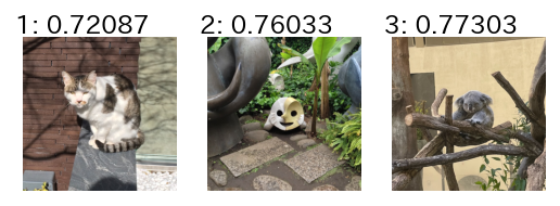
試しにテキストで画像を検索してみます。トップはもちろん猫の写真です。
色々テキストを変えて試してみてください。
text = "猫"
search_image_by_text(text, target_vectors, target_images, closest_n=3)
Out[16]
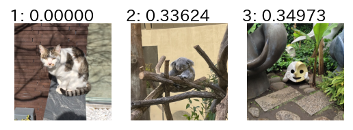
画像で画像を検索してみます。トップは同じ画像なので無視するとして、最も似ているのは「コアラ」で、その次は「午後の日」です。納得感あります。
image = Image.open(f"/content/clip-japanese/sample_images/1.jpeg")
search_image_by_image(image, target_vectors, target_images, closest_n=3)
Out[17]
まとめ、つづく
実際に試しながら使い方を理解できるサンプルコードを用意し、画像とテキストの類似度計算や埋め込みベクトルの計算、類似画像検索の実装方法を解説しました。
ご自身の持っている画像で試してみたり、何か改造して応用してみたり、今回用いた画像とは違う統計的傾向を持った画像を用いてCLIPの新たな傾向分析・考察を行ったりしてみるとより理解が深まると思います。
本シリーズの次回は「いらすとや」さんの画像を検索するシステムの作り方(ゼロショットとファインチューニングの2パターン)について解説する記事になる予定です。