目次
1.はじめに
2.使用データ
3.grib2データを読み込み及び可視化
4.grib2データの可視化結果
5.Netcdf形式での可視化
6.grib2形式とNetcdf版の比較
7.参考文献
はじめに
ここでは、気象庁の解析積雪深をpythonで可視化する。
解析積雪深はgrib2と呼ばれる形式で保存されている。今まではwgrib2を用いて変換し、Netcdfファイルとして使用していたがgrib2をpythonで直接読み込もうと思ったのがきっかけである。
使用環境
Ubuntu 20.04.6 LTS
Python 3.8.10
注意
解析積雪深のgrib2形式に対応するように作成しているので他のgrib2には対応していない。
この記事では、できるだけシンプルにコードを記述するため、読み込みの高速化は考慮していない。
使用データ
- 解析積雪深(grib2)
ここでは、気象庁サンプルデータを用いる(圧縮ファイルを添加して使用)。 - 日本地図(geojson)
japan.geojsonを使わせていただきました。
(日本地図は、cartopyなどのモジュールで描いてもオッケーです。)
grib2データを読み込み及び可視化
# %% --------------
# Import packages
# -----------------
import matplotlib.pyplot as plt
import numpy as np
import matplotlib.colors as mcolors
import geopandas as gpd
from datetime import datetime, timedelta
import matplotlib.style as mplstyle
mplstyle.use("fast")
import lib.read_grib2_ASD as ASD_grib2
import struct
from itertools import repeat
# %% ---------------------
# Define functions (def)
# ------------------------
def set_table(section5):
# Section 5: bytes 15–16 define the maximum data level value
max_level = int.from_bytes(section5[15:17], byteorder="big")
# Read representative values corresponding to each level
table = (
-10, # Representative value for level 0 (Missing Value)
*struct.unpack_from(">" + str(max_level) + "H", section5, 18),
)
return np.array(table, dtype=np.int16)
def decode_runlength(code, hi_level):
level = None # current level for repeating
pwr = 0 # exponent for run-length calculation
for raw in code:
# Normal value: yield as is
if raw <= hi_level:
level = raw
pwr = 0
yield level
else:
# Run-length encoded value
length = (0xFF - hi_level) ** pwr * (raw - (hi_level + 1))
pwr += 1
yield from repeat(level, length)
def load_jmara_grib2(filename):
with open(filename, "rb") as f:
binary = f.read()
pos = 0
len_ = {}
# ---- Section 0 ----
len_["sec0"] = 16
pos += len_["sec0"]
# ---- Section 1 ----
len_["sec1"] = int.from_bytes(binary[pos:pos+4], byteorder="big")
pos += len_["sec1"]
# ---- Section 2 is skipped ----
# ---- Section 3 ----
len_["sec3"] = int.from_bytes(binary[pos:pos+4], byteorder="big")
section3 = binary[pos - 1 : pos + len_["sec3"]]
pos += len_["sec3"]
lon_grid_num = int.from_bytes(section3[31:35], byteorder="big")
lat_grid_num = int.from_bytes(section3[35:39], byteorder="big")
lon_grid_interval = int.from_bytes(section3[64:68], byteorder="big") * 10**-6
lon_grid_interval = round(lon_grid_interval, 4)
lat_grid_interval = int.from_bytes(section3[68:72], byteorder="big") * 10**-6
lat_grid_interval = round(lat_grid_interval, 4)
# ---- Section 4 ----
len_["sec4"] = int.from_bytes(binary[pos:pos+4], byteorder="big")
section4 = binary[pos - 1 : pos + len_["sec4"]]
pos += len_["sec4"]
# ---- Section 5 ----
len_["sec5"] = int.from_bytes(binary[pos:pos+4], byteorder="big")
section5 = binary[pos - 1 : pos + len_["sec5"]]
pos += len_["sec5"]
# Bytes 13–14 define the maximum compression level
highest_level = int.from_bytes(section5[13:15], byteorder="big")
# Generate the level table (mapping levels to representative values)
level_table = set_table(section5)
# ---- Section 6 ----
len_["sec6"] = int.from_bytes(binary[pos:pos+4], byteorder="big")
section6 = binary[pos - 1 : pos + len_["sec6"]]
pos += len_["sec6"]
# ---- Section 7 ----
len_["sec7"] = int.from_bytes(binary[pos:pos+4], byteorder="big")
section7 = binary[pos - 1 : pos + len_["sec7"]]
pos += len_["sec7"]
# Extract run-length encoded data from Section 7
run_length_compressed_columns = section7[6:]
# Decode run-length data
decoded = np.fromiter(
decode_runlength(run_length_compressed_columns, highest_level),
dtype=np.int16
)
# Map levels to representative values and return
return level_table[decoded], lon_grid_num, lat_grid_num,lon_grid_interval,lat_grid_interval
# ==============================
# Input settings
# ==============================
folder = "sample_JMA"
file_name = "Z__C_RJTD_20210118120000_SRF_GPV_Gll5km_Psdlv_ANAL_grib2.bin"
file_path = f"{folder}/{file_name}"
# Display domain
lon_min, lon_max = 118, 150
lat_min, lat_max = 20, 48
snow_depth,lon_grid_num,lat_grid_num,lon_grid_interval,lat_grid_interval =load_jmara_grib2(file_path)
#%%
# ==============================
# Time handling (UTC → JST)
# ==============================
parts = file_name.split("_")
datetime_utc = datetime.strptime(parts[4], "%Y%m%d%H%M%S")
datetime_jst = datetime_utc + timedelta(hours=9)
datetime_jst_str = datetime_jst.strftime("%Y-%m-%d %H:%M JST")
# ==============================
# Load snow depth (cm)
# ==============================
# Divide by 10 to convert the representative data value into a value.
snow_depth = snow_depth.reshape((lat_grid_num, lon_grid_num)) / 10**3 #m
snow_depth = snow_depth *100 #cm
snow_depth[snow_depth < 0] = np.nan
snow_depth =np.flipud(snow_depth)
print(np.unique(snow_depth))
#%%
# ==============================
# Coordinate creation
# ==============================
lon = np.linspace(lon_min, lon_max, lon_grid_num, endpoint=False) +lon_grid_interval / 2
lat = np.linspace(lat_min, lat_max, lat_grid_num, endpoint=False) - lat_grid_interval / 2
X, Y = np.meshgrid(lon, lat)
# ==============================
# Read Japan map
# ==============================
japan_map = gpd.read_file("./geojson/japan.geojson")
jmacolors = np.array(
[
# [242,242,242,1],#white
[160, 210, 255, 1],
[33, 140, 255, 1],
[0, 65, 255, 1],
[250, 245, 0, 1],
[255, 153, 0, 1],
[255, 40, 0, 1],
],
dtype=float,
)
jmacolors[:, :3] /= 256
levels = [0, 5, 20, 50, 100, 150, 200] # 等高線値
cmap = mcolors.ListedColormap(jmacolors[:, :3])
norm = mcolors.BoundaryNorm(levels, cmap.N)
title = "".join(parts[5:10])
fig, ax = plt.subplots(figsize=(8, 8))
extent = [lon.min(), lon.max(), lat.min(), lat.max()]
p = ax.pcolormesh(X, Y, snow_depth, cmap=cmap, norm=norm, shading="auto")
p.cmap.set_over([180 / 256, 0 / 256, 104 / 256])
japan_map.boundary.plot(ax=ax, color="gray", linewidth=0.7)
clb = fig.colorbar(p, ax=ax, shrink=0.5, extend="max",label="cm")
plt.xlim(lon_min, lon_max)
plt.ylim(lat_min, lat_max)
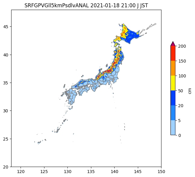
plt.title(f"{title} {datetime_jst_str[:-2]} JST")
plt.show()
grib2データの可視化結果
Netcdf形式での可視化
wgrib2を使って、grib2ファイルをncファイルに変換し、可視化する。
wgrib2については各自でインストールしてほしい。
import geopandas as gpd
import xarray as xr
import numpy as np
from datetime import datetime, timedelta
import matplotlib.pyplot as plt
import matplotlib.colors as mcolors
import os
input_file='./sample_JMA/Z__C_RJTD_20210118120000_SRF_GPV_Gll5km_Psdlv_ANAL_grib2.nc'
df = gpd.read_file('geojson/japan.geojson')
ds = xr.open_dataset(input_file)

# %% ----------------------
# Define functions (date)
# -------------------------
file_name = os.path.basename(input_file)
parts = file_name.split('_')
datetime_UTC_str = parts[4]

# UTC to JST
dt_utc = datetime.strptime(datetime_UTC_str, "%Y%m%d%H%M%S")
dt_jst = dt_utc + timedelta(hours=9)
datetime_jst_str = dt_jst.strftime("%Y%m%d%H%M%S")
# print(datetime_jst_str)


# %% -------------
# Draw a picture
# ----------------
# legend of Analysis snow depth
jmacolors=np.array(
[
    # [242,242,242,1],#white
    [160,210,255,1],
    [33 ,140,255,1],
    [0  ,65 ,255,1],
    [250,245,0,1],
    [255,153,0,1],
    [255,40,0,1],
    # [180,0,104,1],
    # [128, 128, 128, 1]
    ],dtype=float
    )
jmacolors[:,:3] /=256
levels=[0,5,20,50,100,150,200]

lon = ds.longitude
lat = ds.latitude
X, Y = np.meshgrid(lon, lat)

val_name = "var0_1_232_surface"
val = ds[val_name].isel(time = 0)*100
# val[val < 0] = np.nan

fig, ax = plt.subplots(figsize = (8, 8))
cmap = mcolors.ListedColormap(jmacolors)
norm = mcolors.BoundaryNorm(levels, cmap.N)
df.boundary.plot(ax = ax, color = 'gray', linewidth=0.7)

color = np.array([180,0,104,1], dtype=np.float)
color[:3] /= 256
cmap.set_over(color)

p = ax.pcolormesh(X, Y, val, norm = norm, cmap = cmap, shading='auto')
fig.colorbar(p, ax = ax, extend = 'max', shrink=0.5,label="cm")
plt.xlim(118, 150)
plt.ylim(20, 48)
plt.title(f'SRF_GPV_Gll5km_Psdlv_ANAL_{datetime_jst_str} JST nc')
plt.show()
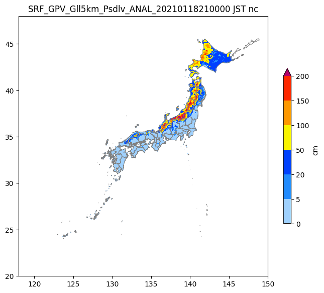
grib2形式とNetcdf版の比較
|
|
Netcdf化するコマンド(Appendix)
wgrib2 ./sample_JMA/Z__C_RJTD_20210118120000_SRF_GPV_Gll5km_Psdlv_ANAL_grib2.bin -netcdf ./sample_JMA/Z__C_RJTD_20210118120000_SRF_GPV_Gll5km_Psdlv_ANAL_grib2.nc
参考文献
1. 気象庁「解析積雪深、解析降雪量」をPythonで読み、作図する(試作版)
2.GPVのサンプルデータ