ニューラルネットワークの重み、バイアス、活性化関数、ニューロン数を変えると、ニューラルネットワーク全体がどう変化するかを可視化します。
以下の3つの活性化関数について検証します。
- シグモイド関数
- ReLU関数
- Mish関数(New!)
実行環境はGoogle Colaboratoryです。
対象者
ニューラルネットワークは学習したけど、いまいちしっくりきてない方。
ニューロンの実装
まずはニューロンを実装しましょう。
ニューロンの処理は、
- 入力値xに重みwを乗算
- 1からバイアスを減算
- 2の結果を活性化関数に渡したものを出力する
ですので、以下のように実装します。
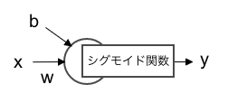
def neuron(x, w, b):
   return activation(w * x - b)
- x:入力値
- w:重み
- b:バイアス
- activation:活性化関数(後ほど定義します)
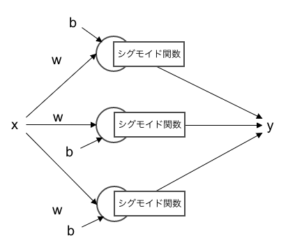
図にすると以下のような感じです。

なるべく、理解の妨げにならないように本来の実装よりもシンプルな構成にしています。
本来のニューラルネットワークの実装よりも以下の点でシンプルにしています。
・出力層では重み1、バイアス0、活性化関数なしの固定とします。(つまり回帰です。)
・複数の入力を受け取る場合、wは配列にすべきですが単純化のため1つの変数で表現します。
シグモイド関数の場合
シグモイド関数を定義し、ニューロン関数も書き換えます。
def sigmoid(x):
  return 1 / (1 + np.exp(-x))

def neuron(x, w, b):
   return sigmoid(w * x - b)
重みの調整
まずは、隠れ層のニューロンが1つの場合を実装します。
重みを調整してどのような変化があるのか確認します。
import numpy as np
import matplotlib.pyplot as plt

def sigmoid(x):
  return 1 / (1 + np.exp(-x))

def neuron(x, w, b):
   return sigmoid(w * x - b)

x = np.arange(-5, 5, 0.1)

# 重み 1 バイアス 0 赤のグラフ
y = neuron(x, 1, 0)
plt.plot(x, y, color="r")

# 重み 0.5 バイアス 0 青のグラフ
y = neuron(x, 0.5, 0)
plt.plot(x, y, color="b")

# 重み 2 バイアス 0 緑のグラフ
y = neuron(x, 2, 0)
plt.plot(x, y, color="g")

plt.ylim(-0.5, 1.5)
plt.show()
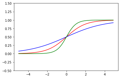
赤が重み1の関数です。
重みを大きくすると急峻なグラフ(緑)に、小さくするとなだらかなグラフ(青)になっていることがわかります。
重みを変更すると傾きが変わるようです。
バイアスの調整
バイアスの影響も確認しましょう。
import numpy as np
import matplotlib.pyplot as plt

def sigmoid(x):
  return 1 / (1 + np.exp(-x))

def neuron(x, w, b):
   return sigmoid(w * x - b)

x = np.arange(-5, 5, 0.1)

# 重み 1 バイアス 0 赤のグラフ
y = neuron(x, 1, 0)
plt.plot(x, y, color="r")

# 重み 1 バイアス -1 青のグラフ
y = neuron(x, 1, -1)
plt.plot(x, y, color="b")

# 重み 1 バイアス 1 緑のグラフ
y = neuron(x, 1, 1)
plt.plot(x, y, color="g")

plt.ylim(-0.5, 1.5)
plt.show()

赤がバイアス1の関数です。
バイアスを大きくすると右(緑)に、小さくすると左(青)に平行移動していることがわかります。
ニューロン数の調整
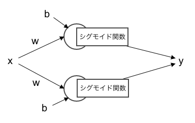
面白いのはここからです。ニューロン数を2つにしてみましょう。
図で表すと以下のような形です。
import numpy as np
import matplotlib.pyplot as plt

def sigmoid(x):
  return 1 / (1 + np.exp(-x))

def neuron(x, w, b):
   return sigmoid(w * x - b)

x = np.arange(-5, 5, 0.1)

# 重み 2 バイアス -2 赤のグラフ
y = neuron(x, 2, -2)
plt.plot(x, y, color="r")

# 重み 0.5 バイアス 1 青のグラフ
y = neuron(x, 0.5, 1)
plt.plot(x, y, color="b")

# 赤の関数と青の関数の和
# 2 * 1の隠れ層 緑のグラフ
y = neuron(x, 2, -2) + neuron(x, 0.5, 1)
plt.plot(x, y, "g")

plt.ylim(-0.5, 2)
plt.show()
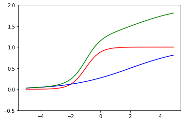
赤の関数が一つ目のニューロン、青の関数がもう一つのニューロンで、2つのニューロンを合わせているニューラルネットワークは緑の関数になります。
ここでもう一個ニューロンを加えて以下のようにしてみましょう。
import numpy as np
import matplotlib.pyplot as plt

def sigmoid(x):
  return 1 / (1 + np.exp(-x))

def neuron(x, w, b):
   return sigmoid(w * x - b)

x = np.arange(-5, 5, 0.1)

# 重み 2 バイアス -2 赤のグラフ
y = neuron(x, 2, -2)
plt.plot(x, y, color="r")

# 重み 0.5 バイアス 1 青のグラフ
y = neuron(x, 0.5, 1)
plt.plot(x, y, color="b")

# 重み 2 バイアス 4 橙のグラフ
y = neuron(x, 2, 4)
plt.plot(x, y, color="orange")

# 赤の関数と青の関数と橙の和
# 3 * 1の隠れ層 緑のグラフ
y = neuron(x, 2, -2) + neuron(x, 0.5, 1) + neuron(x, 2, 4)
plt.plot(x, y, "g")

plt.ylim(-0.5, 3)
plt.show()
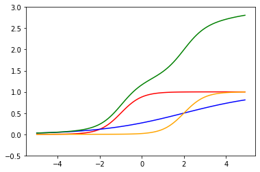
赤、青、橙の関数を合計すると緑の関数になります。
曲がっている関数を合わせることで、どんどんぐにゃぐにゃの関数(表現力の高い関数)になってきました。
ここで橙の関数のニューロンの重みとバイアスをマイナスにしてみます。
どうなるか予想できますか?
import numpy as np
import matplotlib.pyplot as plt

def sigmoid(x):
  return 1 / (1 + np.exp(-x))

def neuron(x, w, b):
   return sigmoid(w * x - b)

x = np.arange(-5, 5, 0.1)

# 重み 2 バイアス -2 赤のグラフ
y = neuron(x, 2, -2)
plt.plot(x, y, color="r")

# 重み 0.5 バイアス 1 青のグラフ
y = neuron(x, 0.5, 1)
plt.plot(x, y, color="b")

# 重み -2 バイアス -4 橙のグラフ
y = neuron(x, -2, -4)
plt.plot(x, y, color="orange")

# 赤の関数と青の関数と橙の和
# 3 * 1の隠れ層 緑のグラフ
y = neuron(x, 2, -2) + neuron(x, 0.5, 1) + neuron(x, -2, -4)
plt.plot(x, y, "g")

plt.ylim(-0.5, 3)
plt.show()
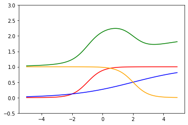
重みを負にすることで、橙の関数の傾きが逆になります。
緑の関数も下方向へ傾きました。
重みで曲線の傾きを変えられる、バイアスで左右に動かせる、ニューロンを増やすことで組み合わせることができる、となると、ニューロンを増やせばどんな関数でも表現できそうな気がしませんか。
ニューラルネットワークの学習は、ニューラルネットワーク関数が学習用データの上を通るように、重みとバイアスを調整することでした。※1
なんとなくニューラルネットワークの学習の過程が見えるような気がしないでしょうか。
※1
回帰の話です。
隠れ層の調整
では、隠れ層を増やして3 + 1のニューラルネットワークを構築してみましょう。

本来、2層目の重みは3つ必要ですが、簡略化のため1つにしています。
層を増やすためにはニューロンの出力値をニューロンに渡せばOKです。
import numpy as np
import matplotlib.pyplot as plt

def sigmoid(x):
  return 1 / (1 + np.exp(-x))

def neuron(x, w, b):
   return sigmoid(w * x - b)

x = np.arange(-5, 5, 0.1)

# 赤の関数と青の関数と橙の和
# 3 * 1の隠れ層 緑のグラフ
y = neuron(x, 2, -2) + neuron(x, 0.5, 1) + neuron(x, -2, -4)
plt.plot(x, y, "g")

# 3 + 1の隠れ層 黒のグラフ
y = neuron(neuron(x, 2, -2) + neuron(x, 0.5, 1) + neuron(x, -2, -4), 1, 0)
plt.plot(x, y, "black")

plt.ylim(0.5, 2.5)
plt.show()
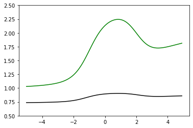
緑の関数を2層目の隠れ層に渡すと黒の関数になります。
どんな異形のグラフができるかと思えば随分とあっさりしてしまいました。
考えてみれば当たり前の話で、シグモイド関数を通すことになるので出力値は0~1の間に収まります。
必然的になだらかなグラフになります。
層が深くなれば深くなるほど、前の方の隠れ層の信号が薄くなってしまいます。
この性質のせいで、シグモイド関数を使ったニューラルネットワークでは層を深くすることができませんでした。
ReLU関数の場合
シグモイド関数の問題を解決したのがReLU関数です。
ReLU関数を定義し、ニューロンも書き換えます。
def relu(x):
    return np.maximum(0, x)

def neuron(x, w, b):
    return relu(w * x - b)
ニューロン数の調整
重み、バイアスの調整は省略してニューロン数を増やしてみましょう。

import numpy as np
import matplotlib.pyplot as plt

def relu(x):
    return np.maximum(0, x)

def neuron(x, w, b):
    return relu(w * x - b)

x = np.arange(-5, 5, 0.1)

# 重み 1 バイアス -2 赤のグラフ
y = neuron(x, 1, -2)
plt.plot(x, y, color="r")

# 重み 0.5 バイアス 0 青のグラフ
y = neuron(x, 0.5, 0)
plt.plot(x, y, color="b")

# 重み -0.5 バイアス -1 橙のグラフ
y = neuron(x, -0.5, -1)
plt.plot(x, y, color="orange")

# 赤の関数と青の関数と橙の関数の和
# 3 * 1の隠れ層 緑のグラフ
y = neuron(x, 1, - 2) + neuron(x, 0.5, 0) + neuron(x, -0.5, -1)
plt.plot(x, y, "g")

plt.ylim(-0.1, 15)
plt.show()

緑が、青、赤、橙の関数の和です。
シグモイド関数と比べるとカクカクしています。
しかも、凹型の関数しか作れません。(作ろうとしてみてください。)
これでは表現力が高いとは言えません。
シグモイド関数の方が活性化関数に適しているのでしょうか。
隠れ層の調整
隠れ層を増やして以下のようにしてみましょう。

シグモイド関数の時のように、なだらかになってしまうでしょうか。
import numpy as np
import matplotlib.pyplot as plt

def relu(x):
    return np.maximum(0, x)

def neuron(x, w, b):
    return relu(w * x - b)

x = np.arange(-5, 5, 0.1)

# 3 * 1の隠れ層 緑のグラフ
y = neuron(x, 1, - 2) + neuron(x, 0.5, 0) + neuron(x, -0.5, -1)
plt.plot(x, y, "g")

# 3 + 1の隠れ層 黒のグラフ
y = neuron(neuron(x, 1, - 2) + neuron(x, 0.5, 0) + neuron(x, -0.5, -1), 1, 0)
plt.plot(x, y, "black")

plt.ylim(-0.1, 10)
plt.show()

緑の関数を2層目の隠れ層に渡したものが黒の関数です。
緑と黒の関数が重なっています。
ReLU関数は0を超えていれば、値をそのまま返すのでグラフの形もそのままになります。(重み1の場合)
シグモイド関数は一層前のニューロンの信号が小さくなってしまっていたので、ReLU関数の方が信号を遠くまで届けることができます。
つまり、ReLU関数はシグモイド関数よりもニューラルネットワークを深くできるといえます。
深層化が進む昨今のニューラルネットワーク事情で、ReLU関数が採用されてきた理由の一つです。
ところで、まだ凹型の関数しか作れていません。
凸型の関数ができれば、凹凸の組み合わせでどんな関数でも作成できそうです。
ここで2層目の隠れ層の重みを負の値にしてみましょう。
import numpy as np
import matplotlib.pyplot as plt

def relu(x):
    return np.maximum(0, x)

def neuron(x, w, b):
    return relu(w * x - b)

x = np.arange(-5, 5, 0.1)

# 3 * 1の隠れ層 緑のグラフ
y = neuron(x, 1, - 2) + neuron(x, 0.5, 0) + neuron(x, -0.5, -1)
plt.plot(x, y, "g")

# 3 + 1の隠れ層 黒のグラフ
y = neuron(neuron(x, 1, - 2) + neuron(x, 0.5, 0) + neuron(x, -0.5, -1), -1, -10)
plt.plot(x, y, "black")

plt.ylim(-0.1, 10)
plt.show()

緑の関数を2層目の隠れ層に渡したものが黒の関数です。
2層目の重みを負にすることによって、グラフを反転させることができました。
ReLU関数でも様々な関数が実現できそうです。
Mish関数
最後に今話題のMish関数を試してみましょう。
Mish関数にはtanh関数が必要なので先に定義しています。
def tanh(x):
    return (np.exp(x) – np.exp(-x)) / (np.exp(x) + np.exp(-x))

def mish(x):
    return x * tanh(np.log(1 + np.exp(x)))

def neuron(x, w, b):
    return mish(w * x - b)
Mish関数のグラフは次のような形になります。

滑らかなReLU関数という印象でしょうか。
一部、負の値を取るのも特徴的です。
ニューロンの調整
さっそくニューロンの数を調整をしてみましょう。
import numpy as np
import matplotlib.pyplot as plt

def tanh(x):
  return (np.exp(x) - np.exp(-x)) / (np.exp(x) + np.exp(-x))

def mish(x):
  return x * tanh(np.log(1 + np.exp(x)))

def neuron(x, w, b):
    return mish(w * x - b)

x = np.arange(-5, 5, 0.1)

# 重み 1 バイアス -2 赤のグラフ
y = neuron(x, 1, -2)
plt.plot(x, y, color="r")

# 重み 0.5 バイアス 0 青のグラフ
y = neuron(x, 0.5, 0)
plt.plot(x, y, color="b")

# 重み -0.5 バイアス -1 橙のグラフ
y = neuron(x, -0.5, -1)
plt.plot(x, y, color="orange")

# 赤の関数と青の関数と橙の関数の和
# 3 * 1の隠れ層 緑のグラフ
y = neuron(x, 1, - 2) + neuron(x, 0.5, 0) + neuron(x, -0.5, -1)
plt.plot(x, y, "g")

plt.ylim(-1, 10)
plt.show()

緑が、青、赤、橙の関数の和です。
元の形がReLU関数と似ているので似たようなグラフをになっています。
違いは滑らかさと負の値でしょうか。
隠れ層の調整
隠れ層を増やしてみましょう。
import numpy as np
import matplotlib.pyplot as plt

def tanh(x):
  return (np.exp(x) - np.exp(-x)) / (np.exp(x) + np.exp(-x))

def mish(x):
  return x * tanh(np.log(1 + np.exp(x)))

def neuron(x, w, b):
    return mish(w * x - b)

x = np.arange(-5, 10, 0.1)

# 3 * 1の隠れ層 緑のグラフ
y = neuron(x, 1, - 2) + neuron(x, 0.5, 0) + neuron(x, -0.5, -1)
plt.plot(x, y, "g")

# 3 + 1の隠れ層 黒のグラフ
y = neuron(neuron(x, 1, - 2) + neuron(x, 0.5, 0) + neuron(x, -0.5, -1), -1, -10)
plt.plot(x, y, "black")

plt.ylim(-1, 10)
plt.show()
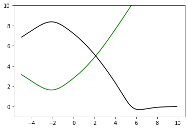
緑の関数を2層目の隠れ層に渡したのが黒の関数です。
Mish関数はReLUの良さである層を深くしても信号が弱まらない特徴と、シグモイド関数の良さである滑らかさを兼ね備えた関数と言えるでしょう。
まとめ
重みの役割
活性化関数の傾きを変化させる働きがある。
バイアスの役割
活性化関数を左右に平行移動させる働きがある。
活性化関数、ニューロン数の役割
活性化関数同士を組み合わせて表現力を高める働きがある。