Chandra の Cas A 画像を FFT して遊ぶ：振幅と位相から見る天体画像の構造

Last updated at 2026-05-23Posted at 2026-05-23

はじめに

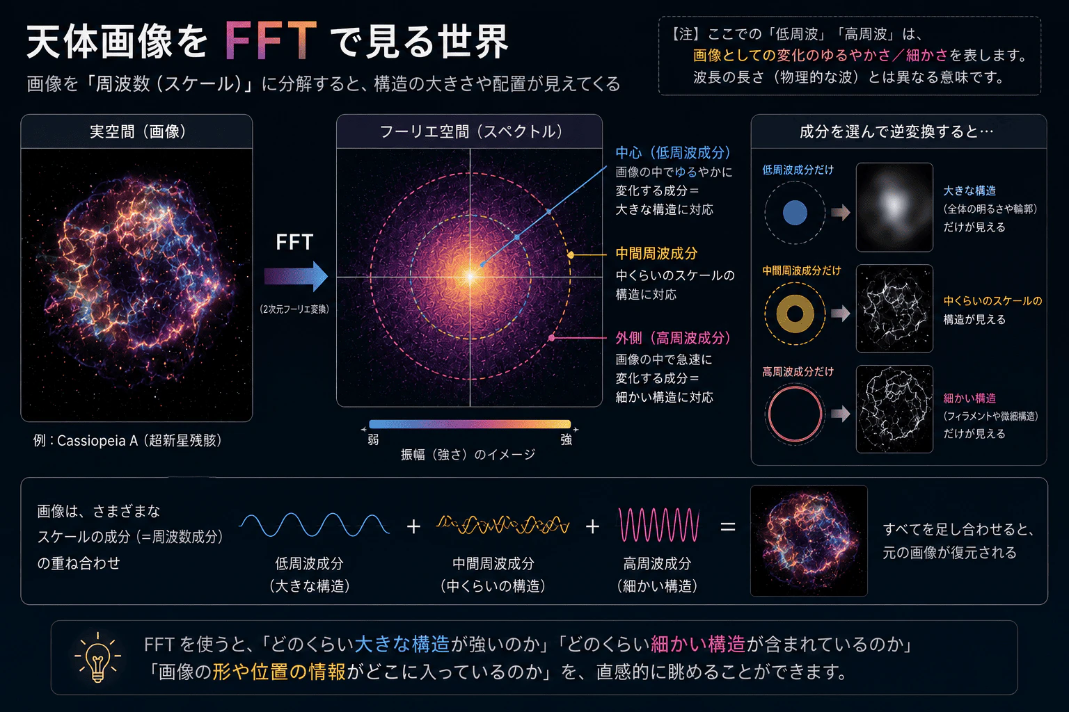
天体画像を見ていると、私たちは自然に「明るいところ」や「細かい構造」に注目します。

たとえば Chandra X線天文衛星で観測された超新星残骸 Cassiopeia A（Cas A）の画像を見ると、shell 状の構造、filament、局所的に明るい knot など、さまざまなスケールの構造が目に入ります。

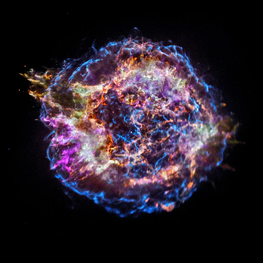
Chandraが観測した Cas A
https://chandra.harvard.edu/photo/2017/casa_life/ より引用

今回は、このような天体画像を Fourier 変換 して遊んでみます。

天体画像解析において Fourier 変換というと、少し数式的で遠いものに感じるかもしれませんが、実際に画像へ FFT をかけてみると、

どのくらい大きな構造が強いのか
どのくらい細かい構造が含まれているのか
画像の形や位置の情報がどこに入っているのか

を、かなり直感的に眺めることができます。

この記事の目的は、コードそのものを詳しく解説することではありません。
コードの細かい説明は最小限にして、実際に画像がどのように変わるのかを見ながら、FFT の振幅と位相の意味を感覚的に理解することを目指します。

この記事では、Chandra の Cas A 画像を題材にして、

FFT の振幅と位相を見る
低周波成分だけで再構成する
高周波成分だけで再構成する
方向を持った Fourier 成分で再構成する
振幅と位相の役割を比べる
ランダム画像を使って振幅と位相の意味を確認する

という流れで見ていきます。

実装コードは Google Colab からもお試しいただけます：
https://colab.research.google.com/drive/1cNcq_Or0lL-sl1Kc-dYlIJPot4giyr3g?usp=sharing

FFT すると何が得られるのか

Fourier 変換の基本的な考え方は、

画像や信号を、さまざまな波の重ね合わせとして表す

というものです。

実際には画像は離散的な pixel データですが、ここではまず直感的なイメージとして「画像を波で分解する」と考えます。

2次元画像を Fourier 変換すると、画像は複素数の配列として表されます。

F(k_x, k_y) = A(k_x, k_y) \exp\{ i \phi(k_x, k_y) \}

ここで、

$A(k_x, k_y)$ が Fourier 振幅
$\phi(k_x, k_y)$ が Fourier 位相

です。

ここで $(k_x, k_y)$ は Fourier 空間での座標で、

大きな $|k|$ → 細かい構造
小さな $|k|$ → 大きな構造

に対応します。

また、$(k_x, k_y)$ の向きは、構造の方向に関する情報も持っています。

振幅は、ざっくり言えば、

どの空間周波数がどれくらい強いか

を表します。

一方、位相は、

それぞれの波がどこで重なって構造を作るか

を表します。

つまり、振幅は「スケールごとの強さ」、位相は「構造の配置」に近い情報を持っています。

画像処理の観点では、画像の特徴は位相に強く含まれることが知られています。
たとえば長橋氏の記事では、2枚の画像の Fourier 振幅と位相を入れ替える例を通して、画像の構造や分布が位相側に強く現れることが説明されています。

参考：画像のフーリエ変換における位相情報はどんな意味

今回はこれを、天体画像、特に Chandra の Cas A 画像で実際に見てみます。

準備：FITS 画像を読み込んで FFT する

まず Cas A の FITS 画像を読み込み、正方形に切り出します。

今回使用する画像は、Chandra Observation ID 4636 の 0.5–7 keV image です。

Google Colab 上で実行する場合は、画像を別途ダウンロードしてアップロードする必要はありません。
内部的に読み込めるように準備しているため、そのまま実行できます。

今回は、FFT の各可視化で同じ入力画像・同じ表示スケールを使います。

そのため、まず最初に、

FITS image の読み込み
Hann window の適用
FFT の計算
Fourier 空間座標の作成
共通関数の定義

などをまとめた共通コードを準備しておきます。

コード量は少し多いですが、この後はこれをベースに各可視化を行っていきます。

共通コードはこちら

import numpy as np
import matplotlib.pyplot as plt

from astropy.io import fits
from scipy.signal.windows import hann
from matplotlib.animation import FuncAnimation
from matplotlib.patches import Circle
from IPython.display import Image


# ======================================================
# common utilities
# ======================================================

def load_cropped_fits_image(filename):
    """
    Read a FITS image and crop it into a square image.
    """

    img = fits.getdata(filename).astype(float)
    img = np.nan_to_num(img, nan=0.0)

    ny, nx = img.shape
    m = min(ny, nx)

    img = img[
        (ny - m) // 2:(ny + m) // 2,
        (nx - m) // 2:(nx + m) // 2
    ]

    return img


def apply_hann_window(img):
    """
    Apply a 2D Hann window to reduce edge effects in FFT.
    """

    m = img.shape[0]

    w = hann(m)
    win2d = np.outer(w, w)

    return img * win2d


def compute_fft(img_win):
    """
    Compute shifted 2D FFT, amplitude, and phase.
    """

    F = np.fft.fft2(img_win)
    F = np.fft.fftshift(F)

    amplitude = np.abs(F)
    phase = np.angle(F)

    return F, amplitude, phase


def make_fourier_coordinates(m):
    """
    Make Fourier-space coordinate maps.
    """

    yy, xx = np.indices((m, m))

    cy, cx = m // 2, m // 2

    kx = xx - cx
    ky = yy - cy

    rr = np.sqrt(kx**2 + ky**2)
    theta = np.arctan2(ky, kx)

    return xx, yy, cx, cy, kx, ky, rr, theta


def make_display_images(img, amplitude):
    """
    Make log-scaled display images and percentile ranges.
    """

    img_disp = np.log10(img + 1)
    amp_disp = np.log10(amplitude + 1)

    img_vmin = np.percentile(img_disp, 5)
    img_vmax = np.percentile(img_disp, 99.7)

    amp_vmin = np.percentile(amp_disp, 5)
    amp_vmax = np.percentile(amp_disp, 99.95)

    return {
        "img_disp": img_disp,
        "amp_disp": amp_disp,
        "img_vmin": img_vmin,
        "img_vmax": img_vmax,
        "amp_vmin": amp_vmin,
        "amp_vmax": amp_vmax,
    }


def reconstruct_from_fft(F_filtered):
    """
    Reconstruct a real-space image from shifted Fourier components.
    """

    img_rec = np.fft.ifft2(
        np.fft.ifftshift(F_filtered)
    ).real

    return img_rec


def make_log_display(img):
    """
    Make a log-scaled image for display.
    Negative values are clipped.
    """

    return np.log10(np.clip(img, 0, None) + 1)


def save_and_show_animation(ani, filename, fps=3):
    """
    Save animation as GIF and display it in Google Colab / Jupyter.
    """

    ani.save(
        filename,
        writer="pillow",
        fps=fps
    )

    plt.close()

    return Image(filename=filename)


# ======================================================
# prepare data
# ======================================================

filename = "casA_image.fits"

img = load_cropped_fits_image(filename)
img_win = apply_hann_window(img)

m = img.shape[0]

F, amplitude, phase_true = compute_fft(img_win)

xx, yy, cx, cy, kx, ky, rr, theta = make_fourier_coordinates(m)

disp = make_display_images(img, amplitude)

img_disp = disp["img_disp"]
amp_disp = disp["amp_disp"]

img_vmin = disp["img_vmin"]
img_vmax = disp["img_vmax"]

amp_vmin = disp["amp_vmin"]
amp_vmax = disp["amp_vmax"]

1. FFT の振幅と位相を見る

まず、元画像、FFT の振幅、FFT の位相を並べて見ます。

コードはこちら

# ======================================================
# plot FFT amplitude and phase
# ======================================================

fig, axs = plt.subplots(1, 3, figsize=(9, 3))

axs[0].imshow(
    img_disp,
    origin="lower",
    cmap="viridis",
    vmin=img_vmin,
    vmax=img_vmax
)

axs[0].set_title("Cas A image")

axs[1].imshow(
    amp_disp,
    origin="lower",
    cmap="magma",
    vmin=amp_vmin,
    vmax=amp_vmax
)

axs[1].set_title("FFT amplitude")

im_phase = axs[2].imshow(
    phase_true,
    origin="lower",
    cmap="twilight",
    vmin=-np.pi,
    vmax=np.pi
)

axs[2].set_title("FFT phase")

plt.colorbar(
    im_phase,
    ax=axs[2],
    fraction=0.046,
    pad=0.04,
    label="radians"
)

# original image
axs[0].set_xlabel("X")
axs[0].set_ylabel("Y")

# Fourier space
for ax in axs[1:]:
    ax.set_xlabel("Fourier X")
    ax.set_ylabel("Fourier Y")

plt.tight_layout()
plt.show()

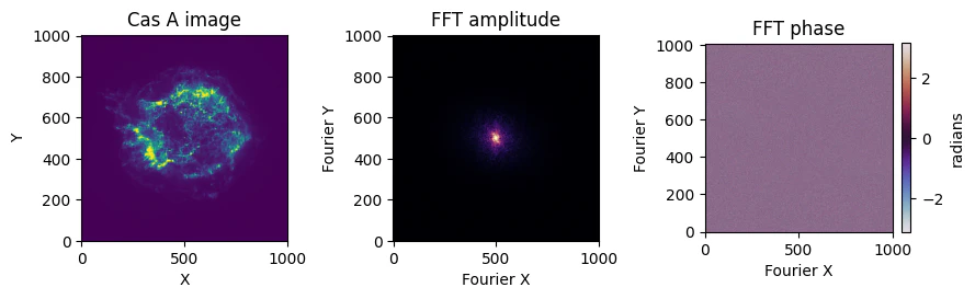
FFT の振幅を見ると、中心付近に強い成分が集中しています。

今回は fftshift を使っているため、ゼロ周波数成分が画像の中心に来るように並べ替えています。
そのため、中心付近は低周波成分、外側は高周波成分に対応します。

つまり、

中心付近 → shell 全体のような大きな構造
外側 → filament や knot のような細かい構造

に対応していると見ることができます。

ここで表示しているのは実空間の $(x, y)$ ではなく、Fourier 空間です。
Fourier 空間には、構造の細かさだけでなく、方向に関する情報も含まれています。

一方で、位相は一見するとランダムな模様に見えます。
ただ、後で見るように、画像の「形」や「配置」に関する情報は、この位相側に強く含まれています。

2. 低周波成分から徐々に戻す

次に、Fourier 空間の中心付近、すなわち低周波成分から順に、少しずつ使う領域を広げながら高周波成分も含めて再構成していきます。

コードはこちら

# ======================================================
# low-pass reconstruction
# ======================================================

def make_lowpass_mask(rr, r):
    return rr <= r


r_inner = np.linspace(2, 40, 15)
r_outer = np.linspace(45, 180, 8)

r_values = np.concatenate([r_inner, r_outer])

mask0 = make_lowpass_mask(rr, r_values[0])

F_filtered = F * mask0
img_rec = reconstruct_from_fft(F_filtered)
img_rec_disp = make_log_display(img_rec)

masked_amp0 = np.where(mask0, amp_disp, np.nan)


fig, axs = plt.subplots(1, 3, figsize=(10, 3), dpi=70)

axs[0].imshow(
    img_disp,
    origin="lower",
    cmap="viridis",
    vmin=img_vmin,
    vmax=img_vmax
)

axs[0].set_title("Cas A image")

im_fft = axs[1].imshow(
    masked_amp0,
    origin="lower",
    cmap="magma",
    vmin=amp_vmin,
    vmax=amp_vmax
)

circle = Circle(
    (cx, cy),
    r_values[0],
    edgecolor="cyan",
    facecolor="none",
    linewidth=2
)

axs[1].add_patch(circle)
axs[1].set_title("Used Fourier components")

im_rec = axs[2].imshow(
    img_rec_disp,
    origin="lower",
    cmap="viridis",
    vmin=img_vmin,
    vmax=img_vmax
)

axs[2].set_title("Reconstructed image")

for ax in axs:
    ax.set_xticks([])
    ax.set_yticks([])

title = fig.suptitle("")
plt.tight_layout()


def update_lowpass(i):

    r = r_values[i]

    mask = make_lowpass_mask(rr, r)

    F_filtered = F * mask
    img_rec = reconstruct_from_fft(F_filtered)
    img_rec_disp = make_log_display(img_rec)

    masked_amp = np.where(mask, amp_disp, np.nan)

    im_fft.set_data(masked_amp)
    circle.set_radius(r)
    im_rec.set_data(img_rec_disp)

    title.set_text(
        f"Low-pass reconstruction: r <= {r:.1f}"
    )

    return im_fft, circle, im_rec, title


ani = FuncAnimation(
    fig,
    update_lowpass,
    frames=len(r_values),
    interval=120,
    blit=False
)

save_and_show_animation(
    ani,
    "casA_fft_lowpass.gif",
    fps=3
)

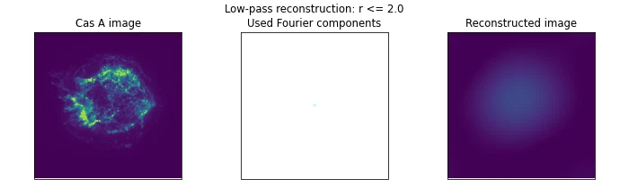
このアニメーションでは、Fourier 空間の中心付近から、徐々に広い領域を使って再構成しています。

最初は低周波成分だけを使っているため、画像全体の大まかな輪郭が見えます。
そこから少しずつ高周波成分を加えることで、filament や knot のような細かい構造が戻ってきます。

3. 高周波成分から徐々に戻す

次に、逆に Fourier 空間の外側（高周波数成分）から順に戻していきます。

コードはこちら

# ======================================================
# high-pass reconstruction
# ======================================================

def make_highpass_mask(rr, r):
    return rr >= r


r_outer = np.linspace(180, 35, 8)
r_inner = np.linspace(30, 0, 16)

r_values = np.concatenate([r_outer, r_inner])

mask0 = make_highpass_mask(rr, r_values[0])

F_filtered = F * mask0
img_rec = reconstruct_from_fft(F_filtered)
img_rec_disp = make_log_display(img_rec)

masked_amp0 = np.where(mask0, amp_disp, np.nan)


fig, axs = plt.subplots(1, 3, figsize=(10, 3), dpi=70)

axs[0].imshow(
    img_disp,
    origin="lower",
    cmap="viridis",
    vmin=img_vmin,
    vmax=img_vmax
)

axs[0].set_title("Cas A image")

im_fft = axs[1].imshow(
    masked_amp0,
    origin="lower",
    cmap="magma",
    vmin=amp_vmin,
    vmax=amp_vmax
)

circle = Circle(
    (cx, cy),
    r_values[0],
    edgecolor="cyan",
    facecolor="none",
    linewidth=2
)

axs[1].add_patch(circle)
axs[1].set_title("Used Fourier components")

im_rec = axs[2].imshow(
    img_rec_disp,
    origin="lower",
    cmap="viridis",
    vmin=img_vmin,
    vmax=img_vmax
)

axs[2].set_title("Reconstructed image")

for ax in axs:
    ax.set_xticks([])
    ax.set_yticks([])

title = fig.suptitle("")
plt.tight_layout()


def update_highpass(i):

    r = r_values[i]

    mask = make_highpass_mask(rr, r)

    F_filtered = F * mask
    img_rec = reconstruct_from_fft(F_filtered)
    img_rec_disp = make_log_display(img_rec)

    masked_amp = np.where(mask, amp_disp, np.nan)

    im_fft.set_data(masked_amp)
    circle.set_radius(r)
    im_rec.set_data(img_rec_disp)

    title.set_text(
        f"High-pass reconstruction: r >= {r:.1f}"
    )

    return im_fft, circle, im_rec, title


ani = FuncAnimation(
    fig,
    update_highpass,
    frames=len(r_values),
    interval=120,
    blit=False
)

save_and_show_animation(
    ani,
    "casA_fft_highpass.gif",
    fps=3
)

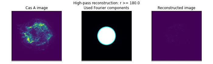
高周波成分だけで再構成すると、元画像の滑らかな明るさ分布というより、

edge
filament
局所的な変化

のような細かい構造が強調されます。

4. 方向を持った Fourier 成分で戻す

Fourier 空間では、周波数の大きさだけでなく、方向も選ぶことができます。

今回は、

低周波成分は常に残す
高周波成分のうち、ある角度方向の成分だけを残す

というマスクを作り、角度を変えながら画像を再構成します。

コードはこちら

# ======================================================
# directional reconstruction
# ======================================================

def angular_difference(theta, theta0):
    """
    Angular difference modulo pi.
    theta and theta + pi are treated as the same direction.
    """

    diff = np.angle(
        np.exp(1j * 2 * (theta - theta0))
    ) / 2

    return np.abs(diff)


def make_directional_mask(
    rr,
    theta,
    theta0,
    dtheta,
    r_low,
    r_min,
    r_max
):
    """
    Keep low-frequency components and directional high-frequency components.
    """

    low_mask = rr <= r_low

    angle_mask = angular_difference(theta, theta0) < dtheta
    radial_mask = (rr >= r_min) & (rr <= r_max)

    directional_mask = angle_mask & radial_mask

    return low_mask | directional_mask


angle_values = np.linspace(0, np.pi, 18)

dtheta = np.deg2rad(10)

r_low = 20
r_min = 15
r_max = 140

mask0 = make_directional_mask(
    rr=rr,
    theta=theta,
    theta0=angle_values[0],
    dtheta=dtheta,
    r_low=r_low,
    r_min=r_min,
    r_max=r_max
)

F_filtered = F * mask0
img_rec = reconstruct_from_fft(F_filtered)
img_rec_disp = make_log_display(img_rec)

masked_amp0 = np.where(mask0, amp_disp, np.nan)


fig, axs = plt.subplots(1, 3, figsize=(10, 3), dpi=70)

axs[0].imshow(
    img_disp,
    origin="lower",
    cmap="viridis",
    vmin=img_vmin,
    vmax=img_vmax
)

axs[0].set_title("Cas A image")

im_fft = axs[1].imshow(
    masked_amp0,
    origin="lower",
    cmap="magma",
    vmin=amp_vmin,
    vmax=amp_vmax
)

axs[1].set_title("Used Fourier components")

im_rec = axs[2].imshow(
    img_rec_disp,
    origin="lower",
    cmap="viridis",
    vmin=img_vmin,
    vmax=img_vmax
)

axs[2].set_title("Reconstructed image")

for ax in axs:
    ax.set_xticks([])
    ax.set_yticks([])

title = fig.suptitle("")
plt.tight_layout()


def update_directional(i):

    theta0 = angle_values[i]

    mask = make_directional_mask(
        rr=rr,
        theta=theta,
        theta0=theta0,
        dtheta=dtheta,
        r_low=r_low,
        r_min=r_min,
        r_max=r_max
    )

    F_filtered = F * mask
    img_rec = reconstruct_from_fft(F_filtered)
    img_rec_disp = make_log_display(img_rec)

    masked_amp = np.where(mask, amp_disp, np.nan)

    im_fft.set_data(masked_amp)
    im_rec.set_data(img_rec_disp)

    title.set_text(
        f"Directional reconstruction: angle = {np.rad2deg(theta0):.1f} deg"
    )

    return im_fft, im_rec, title


ani = FuncAnimation(
    fig,
    update_directional,
    frames=len(angle_values),
    interval=150,
    blit=False
)

save_and_show_animation(
    ani,
    "casA_fft_directional.gif",
    fps=3
)

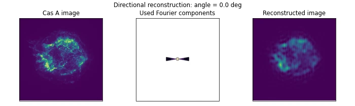
角度を変えることで、画像中の方向性を持った構造の見え方が変わります。
これは、実空間で特定の向きを持つ構造を強調していることに対応します。

Cas A の shell や filament は、完全に同じ方向・同じ強さで広がっているわけではありません。
そのため、方向成分を変えながら見ると、画像の中にある「向きによる構造の違い」を直感的に眺めることができます。

5. 振幅と位相の役割を比べる

ここからが、今回一番面白い部分です。

Fourier 変換後の画像は、

F = A e^{i\phi}

と書けます。

では、振幅と位相のどちらが画像らしさを持っているのでしょうか。

そこで、次の3つを比較します。

case	振幅	位相
original	元画像の振幅	元画像の位相
振幅のみ	元画像の振幅	すべて 0
位相のみ	すべて 1	元画像の位相

つまり、「振幅のみ」では、元画像の振幅をそのまま使い、位相をすべて 0 にします。

一方、「位相のみ」では、元画像の位相をそのまま使い、振幅をすべて 1 にします。

このように整理すると、「片方の情報を使う」と言っても、もう片方をどう扱っているのかが明確になります。

コードはこちら

# ======================================================
# amplitude / phase / reconstruction matrix
# ======================================================

# ------------------------------------------------------
# case 1: original amplitude + original phase
# ------------------------------------------------------

amp_original = amplitude
phase_original = phase_true

F_original = amp_original * np.exp(1j * phase_original)
img_original_rec = reconstruct_from_fft(F_original)

# ------------------------------------------------------
# case 2: original amplitude + zero phase
# ------------------------------------------------------
# This is the "amplitude only" case.
# The phase is set to zero everywhere.

amp_amp_only = amplitude
phase_amp_only = np.zeros_like(phase_true)

F_amp_only = amp_amp_only * np.exp(1j * phase_amp_only)
img_amp_only = reconstruct_from_fft(F_amp_only)

# shift only for display
img_amp_only = np.fft.fftshift(img_amp_only)

# ------------------------------------------------------
# case 3: unit amplitude + original phase
# ------------------------------------------------------
# This is the "phase only" case.
# The amplitude is set to unity everywhere.

amp_phase_only = np.ones_like(amplitude)
phase_phase_only = phase_true

F_phase_only = amp_phase_only * np.exp(1j * phase_phase_only)
img_phase_only = reconstruct_from_fft(F_phase_only)

# ======================================================
# display images
# ======================================================

amp_original_disp = np.log10(amp_original + 1)
amp_amp_only_disp = np.log10(amp_amp_only + 1)
amp_phase_only_disp = np.log10(amp_phase_only + 1)

img_original_rec_disp = make_log_display(img_original_rec)
img_amp_only_disp = make_log_display(img_amp_only)

# phase-only reconstruction has positive and negative values.
# Show absolute value for intuitive visualization.
img_phase_only_disp = np.log10(np.abs(img_phase_only) + 1)

# ------------------------------------------------------
# display ranges
# ------------------------------------------------------

amp_vmin = np.percentile(amp_original_disp, 5)
amp_vmax = np.percentile(amp_original_disp, 99.95)

rec_vmin = np.percentile(img_original_rec_disp, 5)
rec_vmax = np.percentile(img_original_rec_disp, 99.7)

amp_only_vmin = np.percentile(img_amp_only_disp, 5)
amp_only_vmax = np.percentile(img_amp_only_disp, 99.7)

phase_only_vmin = np.percentile(img_phase_only_disp, 5)
phase_only_vmax = np.percentile(img_phase_only_disp, 99.7)

# ======================================================
# figure
# ======================================================

fig, axs = plt.subplots(3, 3, figsize=(9, 9))

# ======================================================
# row 1: original amplitude + original phase
# ======================================================

axs[0, 0].imshow(
    amp_original_disp,
    origin="lower",
    cmap="magma",
    vmin=amp_vmin,
    vmax=amp_vmax
)

axs[0, 0].set_title("Amplitude")
axs[0, 0].set_ylabel("Original")

axs[0, 1].imshow(
    phase_original,
    origin="lower",
    cmap="twilight",
    vmin=-np.pi,
    vmax=np.pi
)

axs[0, 1].set_title("Phase")

axs[0, 2].imshow(
    img_original_rec_disp,
    origin="lower",
    cmap="viridis",
    vmin=rec_vmin,
    vmax=rec_vmax
)

axs[0, 2].set_title("Reconstruction")

# ======================================================
# row 2: amplitude only
# ======================================================

axs[1, 0].imshow(
    amp_amp_only_disp,
    origin="lower",
    cmap="magma",
    vmin=amp_vmin,
    vmax=amp_vmax
)

axs[1, 0].set_ylabel("Amplitude only")

axs[1, 1].imshow(
    phase_amp_only,
    origin="lower",
    cmap="twilight",
    vmin=-np.pi,
    vmax=np.pi
)

axs[1, 2].imshow(
    img_amp_only_disp,
    origin="lower",
    cmap="viridis",
    vmin=amp_only_vmin,
    vmax=amp_only_vmax
)

# ======================================================
# row 3: phase only
# ======================================================

axs[2, 0].imshow(
    amp_phase_only_disp,
    origin="lower",
    cmap="magma",
    vmin=amp_vmin,
    vmax=amp_vmax
)

axs[2, 0].set_ylabel("Phase only")

axs[2, 1].imshow(
    phase_phase_only,
    origin="lower",
    cmap="twilight",
    vmin=-np.pi,
    vmax=np.pi
)

axs[2, 2].imshow(
    img_phase_only_disp,
    origin="lower",
    cmap="viridis",
    vmin=phase_only_vmin,
    vmax=phase_only_vmax
)

# ======================================================
# style
# ======================================================

for ax in axs.ravel():
    ax.set_xticks([])
    ax.set_yticks([])

plt.tight_layout()
plt.show()

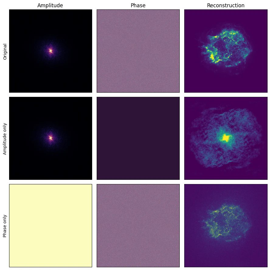
1行目: 元画像の振幅 + 元画像の位相 → 再構成画像
2行目: 元画像の振幅 + ゼロ位相 → 再構成画像
3行目: 一様な振幅 + 元画像の位相 → 再構成画像

列は、

振幅
位相
再構成画像

実際に再構成すると、「振幅のみ」でも何らかの広がりやスケール感は残ります。
しかし、Cas A らしい shell や filament の配置はかなり崩れます。

一方で「位相のみ」では、振幅をすべて 1 にしているにもかかわらず、Cas A の構造がかなり見えてきます。

これはとても面白い結果です。

振幅は、

どの空間周波数が強いか

を持っています。

しかし位相は、

その周波数成分がどこで重なって画像構造を作るか

を持っています。

そのため、画像の「形」や「特徴」は位相に強く残ります。

6. 振幅固定・位相固定でランダム画像を作る

さらに一歩進めて、ランダム成分を使った実験もしてみます。

ここでは、

Cas A の振幅を固定し、位相だけランダムにする
Cas A の位相を固定し、振幅だけランダムにする

という2種類の画像を作ります。

前者は、

周波数ごとの強さは Cas A と同じだが、波の重なり方はランダム

という画像です。

後者は、

波の重なり方は Cas A と同じだが、周波数ごとの強さはランダム

という画像です。

コードはこちら

# ======================================================
# random reconstructions with fixed amplitude or fixed phase
# ======================================================

n_random = 3

rng = np.random.default_rng(1)


def make_random_fourier_components(shape, rng):
    """
    Generate random Fourier amplitude and phase from a random real image.

    Using a random real image helps keep the Hermitian symmetry,
    so the inverse FFT remains approximately real.
    """

    random_img = rng.normal(size=shape)

    F_random = np.fft.fft2(random_img)
    F_random = np.fft.fftshift(F_random)

    amplitude_random = np.abs(F_random)
    phase_random = np.angle(F_random)

    return amplitude_random, phase_random


def normalize_amplitude(amplitude_input, amplitude_reference):
    """
    Normalize random amplitude so that its total power is comparable
    to the reference amplitude.
    """

    scale = np.sum(amplitude_reference) / np.sum(amplitude_input)

    return amplitude_input * scale


# ======================================================
# make random reconstructions
# ======================================================

fixed_amplitude_images = []
fixed_phase_images = []

for i in range(n_random):

    amplitude_random, phase_random = make_random_fourier_components(
        shape=img.shape,
        rng=rng
    )

    amplitude_random = normalize_amplitude(
        amplitude_input=amplitude_random,
        amplitude_reference=amplitude
    )

    # --------------------------------------------------
    # fixed amplitude + random phase
    # --------------------------------------------------
    # The frequency strength is fixed to the original Cas A.
    # Only the phase is randomized.

    F_fixed_amplitude = amplitude * np.exp(1j * phase_random)

    img_fixed_amplitude = reconstruct_from_fft(F_fixed_amplitude)

    fixed_amplitude_images.append(img_fixed_amplitude)

    # --------------------------------------------------
    # random amplitude + fixed phase
    # --------------------------------------------------
    # The phase is fixed to the original Cas A.
    # Only the amplitude is randomized.

    F_fixed_phase = amplitude_random * np.exp(1j * phase_true)

    img_fixed_phase = reconstruct_from_fft(F_fixed_phase)

    fixed_phase_images.append(img_fixed_phase)


# ======================================================
# display images
# ======================================================

fixed_amplitude_disp = [
    np.log10(np.abs(x) + 1)
    for x in fixed_amplitude_images
]

fixed_phase_disp = [
    np.log10(np.abs(x) + 1)
    for x in fixed_phase_images
]

# Use common display ranges for each row.
fixed_amplitude_vmin = np.percentile(
    np.concatenate([x.ravel() for x in fixed_amplitude_disp]),
    5
)

fixed_amplitude_vmax = np.percentile(
    np.concatenate([x.ravel() for x in fixed_amplitude_disp]),
    99.7
)

fixed_phase_vmin = np.percentile(
    np.concatenate([x.ravel() for x in fixed_phase_disp]),
    5
)

fixed_phase_vmax = np.percentile(
    np.concatenate([x.ravel() for x in fixed_phase_disp]),
    99.7
)


# ======================================================
# figure
# ======================================================

fig, axs = plt.subplots(2, n_random + 1, figsize=(14, 7))

# ------------------------------------------------------
# row 1: fixed amplitude + random phase
# ------------------------------------------------------

axs[0, 0].imshow(
    img_disp,
    origin="lower",
    cmap="viridis",
    vmin=img_vmin,
    vmax=img_vmax
)

axs[0, 0].set_title("Original Cas A")
axs[0, 0].set_ylabel("Fixed amplitude\nrandom phase")

for i in range(n_random):

    axs[0, i + 1].imshow(
        fixed_amplitude_disp[i],
        origin="lower",
        cmap="viridis",
        vmin=fixed_amplitude_vmin,
        vmax=fixed_amplitude_vmax
    )

    axs[0, i + 1].set_title(f"Random {i + 1}")


# ------------------------------------------------------
# row 2: random amplitude + fixed phase
# ------------------------------------------------------

axs[1, 0].imshow(
    img_disp,
    origin="lower",
    cmap="viridis",
    vmin=img_vmin,
    vmax=img_vmax
)

axs[1, 0].set_title("Original Cas A")
axs[1, 0].set_ylabel("Random amplitude\nfixed phase")

for i in range(n_random):

    axs[1, i + 1].imshow(
        fixed_phase_disp[i],
        origin="lower",
        cmap="viridis",
        vmin=fixed_phase_vmin,
        vmax=fixed_phase_vmax
    )

    axs[1, i + 1].set_title(f"Random {i + 1}")


# ------------------------------------------------------
# style
# ------------------------------------------------------

for ax in axs.ravel():
    ax.set_xticks([])
    ax.set_yticks([])

plt.tight_layout()
plt.show()

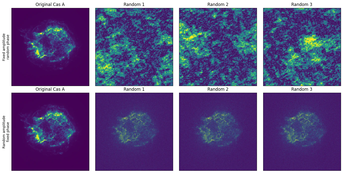
上段: 振幅固定 + ランダム位相
下段: ランダム振幅 + 位相固定
それぞれ random seed を変えて 3 例ほど表示

この比較をすると、振幅と位相の違いがかなり直感的にわかります。

振幅固定・位相ランダムの画像では、Cas A と同じ power spectrum 的な性質を持つため、スケール感や texture はある程度似ます。
しかし、Cas A の shell や filament の配置は崩れます。

一方で、位相固定・振幅ランダムの画像では、振幅を変えているにもかかわらず、Cas A らしい構造が残りやすくなります。

もちろん、これは「位相だけで物理量が完全にわかる」という意味ではありません。

X線天文学では、

カウント数
エネルギー帯
露光補正
PSF
背景
統計誤差

などが非常に重要です。

ただし、画像の構造情報という観点では、位相が非常に大きな役割を持っていることがわかります。

天体解析とのつながり：周波数成分を見るということ

今回は簡単な FFT の紹介にとどめましたが、実際の天体画像解析でも、空間周波数で画像を見る考え方はとても重要です。

たとえば Chandra の解析でよく使われる wavdetect は、Mexican Hat wavelet を用いて局所的な構造を検出するツールです。

wavdetect は Fourier 変換そのものではありませんが、

画像を空間スケールごとに分解して見る

という意味では、今回の low-pass / high-pass reconstruction と近い発想を持っています。

wavdetect については、こちらの記事が非常にわかりやすく参考になります。

また、Fourier 成分を見る考え方は、単に画像を見やすくするだけでなく、天体画像の構造を定量的に調べるときにも使われます。

たとえば Saha et al. (2021) では、Cas A の電波画像と Chandra X線画像に対して角度パワースペクトルを調べ、構造の空間スケールや、乱流的な揺らぎとの関係を議論しています。

https://doi.org/10.1093/mnras/stab446

このように、今回の記事で見た「画像を空間周波数で見る」という考え方は、実際の天体画像解析でも使われています。

さらに、Fourier 成分を見る考え方は、電波干渉計や VLBI にも深くつながっています。

最近、量子光学と量子 VLBI をつなぐ記事の中でも、Van Cittert–Zernike theorem と Fourier 変換の関係が紹介されていました。

VCZ theorem では、天体の brightness distribution と visibility が Fourier 変換で結びつきます。

つまり、

画像の Fourier 成分を見る

という考え方は、実は天文学でもかなり本質的だと思います。

まとめ

今回は、Chandra の Cas A 画像を題材にして、FFT で遊んでみました。

やったことは、

FFT の振幅と位相を見る
low-pass reconstruction で大きな構造を見る
high-pass reconstruction で細かい構造を見る
directional reconstruction で方向性を持つ構造を見る
「振幅のみ」/「位相のみ」で画像構造の情報がどこにあるかを見る
振幅固定・位相固定のランダム画像で、その違いを確認する

という内容です。

特に面白いのは、「位相のみ」の再構成でも Cas A らしい構造がかなり残ることです。

これは、画像の特徴が Fourier 位相に強く含まれるという画像処理の考え方と対応しています。

天体画像解析では、最終的には物理量、統計、装置応答、PSF まで含めて丁寧に扱う必要があります。

ただ、その前段階として、画像を空間周波数で見る感覚を持っておくと、wavelet 解析、フィルタリング、PSF、deconvolution 解析などへの理解がつながりやすくなります。

FFT は少し数学っぽく見えますが、実際には、

画像の中にどんなスケールの構造があるのかを見るための道具

だと思うと、かなり直感的に扱えるようになります。

Cas A のように複雑で美しい天体画像を使うと、その感覚がより掴みやすいかもしれません。

参考

長橋宏
「画像のフーリエ変換における位相情報はどんな意味」
https://www.jstage.jst.go.jp/article/itej1997/54/10/54_10_1408/_pdf
Saha et al. (2021)
"The auto- and cross-angular power spectrum of the Cas A supernova remnant in radio and X-ray"
https://doi.org/10.1093/mnras/stab446

You get articles that match your needs
You can efficiently read back useful information
You can use dark theme

What you can do with signing up