第一回：
https://qiita.com/s_zh/items/3b183e258bcd6506e8cb
第二回：
https://qiita.com/s_zh/items/1b193758965a491e79bc
第三回：
https://qiita.com/s_zh/items/75b129f8279e290fe705

今回使うNode Embedding LibraryはNeo4j Sandboxには搭載されておらず、実行するには無料のNeo4j DesktopかComunity版をインストールする必要があります。

Node Embeddingについて

今まではPageRankやLouvainアルゴリズムを使って重要なノードを見つけたり、つながりの強いグループを見つけたりしました。

一方でノードやリレーションシップの特徴量を抽出できれば、従来の機械学習手法を適応しやすくなります。例えばアカウントをさまざまな視点で分類したり、属するグループだけではなくアカウント間の関係を数値化したり、グループ間の関係を数値化したり、可視化したりするなど行うことができます。

特別に他の特徴量を用意しなくても繋がりさえあれば全体から見た場合の特徴量を使うことができるのはカラム志向に対してグラフ志向でデータを捉える利点の１つだと思います。

Node Embeddingはノードの特徴を表すベクトルを算出します。NLPで有名なWord2Vecも一種のNode Embeddingとして捉えることもできます。基本的な考え方としてはノード間のリンクを再現できるように各ノードにベクトルを割り当てます。

今回はNeo4j Data Science LibraryのNode Embeddingについて見てみます。

Neo3j Graph Data Science LibraryとNode Embedding

Neo4j Graph Data Science Libraryはα版でNode Embeddingアルゴリズムを提供しています。

アルゴリズムの種類としてはWord2Vec流のNode2Vec、ノード属性を活用できるグラフニューラルネットワーク流のGraphSage、そして高速のRandom Projectionが用意されています。

ここではNode2Vecを使います。

Node Embeddingの算出

グラフは前回まで使っていた政治家のみのネットワークを流用します。
作成する場合は次のように行います。

CALL gds.graph.create.cypher( 
    'follow-net-politicians', 
    'MATCH (g:Group)--(u:User) WITH DISTINCT u RETURN id(u) AS id', 
    'MATCH (:Group)--(u:User)-[r:FOLLOW]->(u2:User)--(:Group) WITH DISTINCT r, u, u2 RETURN id(u) AS source, id(u2) AS target')

10次元（node2vec）と3次元(node2vec3d)、4次元(node2vec4d)のEmbeddingをそれぞれ計算して、属性として保存します。
次元数の選び方に関しては、一般的なWord2Vecは数十万〜数百万の単語（ノード）を100~300次元へ落とし込むのが１つの目安になります。
今回は300程度のアカウントなので、あまり高次元にすると過学習が起きやすくなってしまいます。

CALL gds.alpha.node2vec.write('follow-net-politicians', 
{embeddingSize: 10,
writeProperty: 'node2vec'})

CALL gds.alpha.node2vec.write('follow-net-politicians', 
{embeddingSize: 3,
writeProperty: 'node2vec3d'})

CALL gds.alpha.node2vec.write('follow-net-politicians', 
{embeddingSize: 4,
writeProperty: 'node2vec4d'})

検証

作成したEmbeddingを見てみます

import plotly.express as px
import numpy as np

from neo4j import GraphDatabase
from tqdm.notebook import tqdm
import json

import pandas as pd

auth_path = './data/neo4j_graph/auth.json'
with open(auth_path, 'r') as f:
    auth = json.load(f)

# ローカルの場合は通常 uri: bolt(or neo4j)://localhost:7687, user: neo4j, pd: 設定したもの
# サンドボックスの場合は作成画面から接続情報が見られます
uri = 'neo4j://localhost:7687'
driver = GraphDatabase.driver(uri=uri, auth=(auth['user'], auth['pd']))

# Sandboxの場合はこんな感じ
# uri = 'bolt://54.175.38.249:35275'
# driver = GraphDatabase.driver(uri=uri, auth=('neo4j', 'spray-missile-sizing'))

3d

dim_no = 3

with driver.session() as session:
    res = session.run('''
    MATCH (u:User)--(:Group)
    WITH DISTINCT u
    RETURN u.screenName as screen_name, u.name as name, u.louvainCommunityUndirected as community, u.node2vec3d as embedding
    ''')

res_df = pd.DataFrame([r.data() for r in res])
res_df.head()

	screen_name	name	community	embedding
0	tadamori_oshima	大島理森	3	[-0.20086176693439484, 0.9452930688858032, 1.1...
1	YAMASHITA_OK	山下たかし	3	[-0.3143966794013977, 0.4608628451824188, 1.31...
2	andouhiroshi	あんどう裕(ひろし)衆議院議員(自民党京都６区 )	3	[-0.03988641873002052, 0.4570828974246979, 1.2...
3	jimin_koho	自民党広報	3	[-0.564670205116272, 0.5222573280334473, 1.403...
4	Matsukawa_Rui	松川るい =自民党=	3	[-0.5284397602081299, 0.6824808716773987, 1.36...

Node Embeddingは関係のの近いノードを近い方向に配置し、ノードの重要性（出現頻度など）を絶対値に反映しているので、可視化する時にすべてのベクトルの大きさを１に揃えたほうがわかりやすいです。

def renorm_vector(v):
    norm = np.sqrt(sum([c**2 for c in v]))
    return np.array(v) / norm

ax_columns = ['x{}'.format(i) for i in range(1, dim_no+1)]

# res_df[ax_columns] = res_df.embedding.apply(pd.Series)

res_df[ax_columns] = res_df.embedding.apply(lambda x: pd.Series(renorm_vector(x)))

res_df.head()

	screen_name	name	community	embedding	x1	x2	x3
0	tadamori_oshima	大島理森	3	[-0.20086176693439484, 0.9452930688858032, 1.1...	-0.132467	0.623415	0.770588
1	YAMASHITA_OK	山下たかし	3	[-0.3143966794013977, 0.4608628451824188, 1.31...	-0.220553	0.323301	0.920235
2	andouhiroshi	あんどう裕(ひろし)衆議院議員(自民党京都６区 )	3	[-0.03988641873002052, 0.4570828974246979, 1.2...	-0.030714	0.351969	0.935508
3	jimin_koho	自民党広報	3	[-0.564670205116272, 0.5222573280334473, 1.403...	-0.352781	0.326283	0.876975
4	Matsukawa_Rui	松川るい =自民党=	3	[-0.5284397602081299, 0.6824808716773987, 1.36...	-0.327500	0.422967	0.844892

ここで比較するために以前計算していたクラスタリングを取得しています。
各クラスタに入っているノード数は次のようになります。

res_df.community = res_df.community.astype('category')
res_df.community.value_counts()

174    127
3      107
169     66
120     29
257     17
Name: community, dtype: int64

fig = px.scatter_3d(res_df,  
                    x="x1",  
                    y="x2",   
                    z='x3', 
                    text="name",  
                    color='community',  
                    log_x=False,  
                    size_max=60)

fig.update_traces(textposition='top center')

fig.update_layout(
    height=800,
    title_text=''
)

fig.show()

# plotを保存する場合
html_path = './data/neo4j_graph/politician_03_3dembedding.html'
with open(html_path, 'w') as f:
    f.write(fig.to_html())

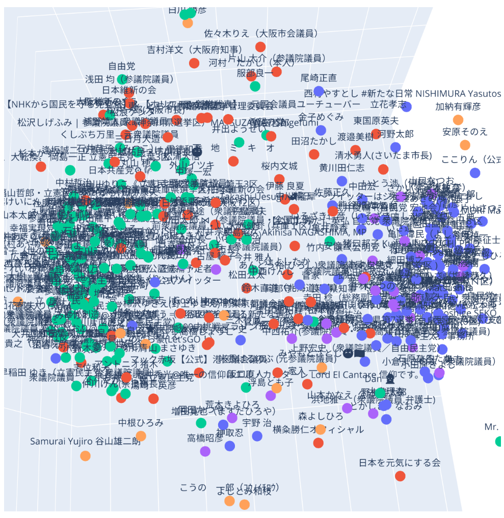
おおむね自民党系と民主党系が左右に固まり、維新系が真ん中にある構図が変わりませんでした。
一方でマイナークラスタはトップ３に埋もれる形になりました。
これは元データに対して次元圧縮をしすぎたため、表現力が足りないためと思われます。

# figf = px.data.gapminder().query("year==2007 and continent=='Americas'")

# fig = px.scatter(res_df,  
#                  x="x1", 
#                  y="x2", 
#                  text="name", 
#                  color='community', 
#                  log_x=False, 
#                  size_max=60)

# fig.update_traces(textposition='top center')

# fig.update_layout(
#     height=800,
#     title_text=''
# )

# fig.show()

4d

では4dでどうなるかをみてみます。

dim_no = 4

with driver.session() as session:
    res = session.run('''
    MATCH (u:User)--(:Group)
    WITH DISTINCT u
    RETURN u.screenName as screen_name, u.name as name, u.louvainCommunityUndirected as community, u.node2vec4d as embedding
    ''')

res_df = pd.DataFrame([r.data() for r in res])
res_df.head()

	screen_name	name	community	embedding
0	tadamori_oshima	大島理森	3	[-0.9669536352157593, -0.4772112965583801, -0....
1	YAMASHITA_OK	山下たかし	3	[-0.944596529006958, -0.29907843470573425, -0....
2	andouhiroshi	あんどう裕(ひろし)衆議院議員(自民党京都６区 )	3	[-0.9364525675773621, -0.093632273375988, -0.8...
3	jimin_koho	自民党広報	3	[-1.0234124660491943, -0.5828015208244324, -0....
4	Matsukawa_Rui	松川るい =自民党=	3	[-0.9714489579200745, -0.48148995637893677, -0...

def renorm_vector(v):
    norm = np.sqrt(sum([c**2 for c in v]))
    return np.array(v) / norm

ax_columns = ['x{}'.format(i) for i in range(1, dim_no+1)]

# res_df[ax_columns] = res_df.embedding.apply(pd.Series)
res_df[ax_columns] = res_df.embedding.apply(lambda x: pd.Series(renorm_vector(x)))

res_df.community = res_df.community.astype('category')

res_df.head()

	screen_name	name	community	embedding	x1	x2	x3	x4
0	tadamori_oshima	大島理森	3	[-0.9669536352157593, -0.4772112965583801, -0....	-0.626852	-0.309364	-0.545948	-0.461835
1	YAMASHITA_OK	山下たかし	3	[-0.944596529006958, -0.29907843470573425, -0....	-0.678253	-0.214749	-0.628372	-0.314651
2	andouhiroshi	あんどう裕(ひろし)衆議院議員(自民党京都６区 )	3	[-0.9364525675773621, -0.093632273375988, -0.8...	-0.736264	-0.073616	-0.657714	-0.141094
3	jimin_koho	自民党広報	3	[-1.0234124660491943, -0.5828015208244324, -0....	-0.691638	-0.393866	-0.530964	-0.290831
4	Matsukawa_Rui	松川るい =自民党=	3	[-0.9714489579200745, -0.48148995637893677, -0...	-0.671192	-0.332670	-0.580522	-0.319101

fig = px.scatter_3d(res_df,  
                    x="x1",  
                    y="x2",   
                    z='x4', 
                    text="name",  
                    color='community',  
                    log_x=False,  
                    size_max=60)

fig.update_traces(textposition='top center')

fig.update_layout(
    height=800,
    title_text=''
)

fig.show()

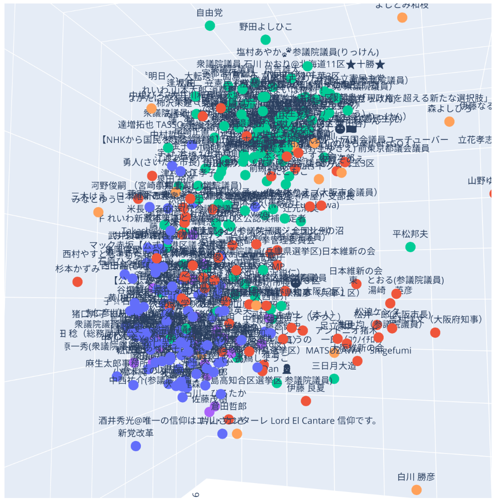
角度を変えて

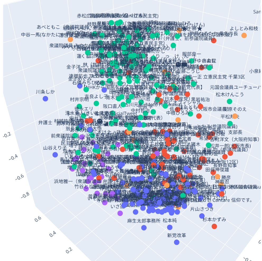
自民系は比較的に固まっていて、民主形はかなり広がりがあり、維新系は自民寄りになっていることが見て取れます。

10d

10dのEmbeddingでクラスタリングしてみます。

from sklearn.cluster import KMeans

with driver.session() as session:
    res = session.run('''
    MATCH (u:User)--(:Group)
    WITH DISTINCT u
    RETURN u.screenName as screen_name, u.name as name, u.louvainCommunityUndirected as community, u.node2vec as embedding
    ''')

res_df = pd.DataFrame([r.data() for r in res])

ax_columns = ['x{}'.format(i) for i in range(1, 11)]

# res_df[ax_columns] = res_df.embedding.apply(pd.Series)

res_df[ax_columns] = res_df.embedding.apply(lambda x: pd.Series(renorm_vector(x)))

res_df.head()

	screen_name	name	community	embedding	x1	x2	x3	x4	x5	x6	x7	x8	x9	x10
0	tadamori_oshima	大島理森	3	[0.8451248407363892, -0.3527873158454895, 0.79...	0.461382	-0.192599	0.433067	-0.204804	-0.220397	-0.109164	0.262750	0.550687	-0.237711	-0.176773
1	YAMASHITA_OK	山下たかし	3	[-0.21574953198432922, -0.9915562868118286, 0....	-0.103789	-0.477001	0.165211	-0.106283	-0.260988	-0.330459	0.587693	0.288013	-0.341218	0.032010
2	andouhiroshi	あんどう裕(ひろし)衆議院議員(自民党京都６区 )	3	[0.48249784111976624, -0.26339074969291687, -0...	0.340378	-0.185809	-0.154462	-0.271198	-0.215974	-0.281920	0.519558	0.533754	-0.059092	-0.260310
3	jimin_koho	自民党広報	3	[0.44367820024490356, -0.663674533367157, 0.38...	0.236184	-0.353295	0.203981	-0.113193	-0.199367	-0.334902	0.628517	0.415378	-0.167158	-0.132505
4	Matsukawa_Rui	松川るい =自民党=	3	[0.19990792870521545, -0.42390283942222595, 0....	0.115597	-0.245123	0.126030	-0.102652	-0.334126	-0.305738	0.538014	0.570700	-0.282578	0.002598

res_df.community = res_df.community.astype('category')
res_df.community.value_counts()

174    127
3      107
169     66
120     29
257     17
Name: community, dtype: int64

Louvainと比較するためにクラス多数を同じ５とします。

k_m = KMeans(n_clusters=5)

embedding_arr = np.array([l for l in res_df.embedding])
embedding_arr.shape

(346, 10)

k_m.fit_predict(embedding_arr)
res_df['k_community'] = res_df.embedding.apply(lambda x: k_m.predict(np.array(x).reshape(1, -1))[0])

for i in res_df.k_community.value_counts().items():
    print(i)
    print(res_df[res_df.k_community == i[0]].community.value_counts())

(0, 130)
174    110
257      9
169      9
3        2
120      0
Name: community, dtype: int64
(1, 117)
3      100
169     12
257      2
174      2
120      1
Name: community, dtype: int64
(2, 62)
169    43
174    12
257     4
120     2
3       1
Name: community, dtype: int64
(3, 35)
120    26
3       4
257     2
169     2
174     1
Name: community, dtype: int64
(4, 2)
174    2
257    0
169    0
120    0
3      0
Name: community, dtype: int64

概ね自民、民主、維新系のまま、すこし趣の違う感じになりました。

クラスタ数について

Embeddingしてからクラスタリングを行う利点のひとつはクラスタ数を調整できることです。
ここでは各クラス多数におけるフィット具合を見てみます。

import matplotlib.pyplot as plt

models = []
for i in tqdm(range(2, 30)):
    k_m = KMeans(n_clusters=i)
    k_m.fit(embedding_arr)
    models.append(k_m)

HBox(children=(IntProgress(value=0, max=28), HTML(value='')))

x = [i for i in range(2, 30)]
y = np.array([k.inertia_ for k in models])
# plt.plot(x, y)
# plt.plot([i for i in range(2, 15)], np.log(np.array([k.inertia_ for k in models])))

px.line(x=x, y=y)

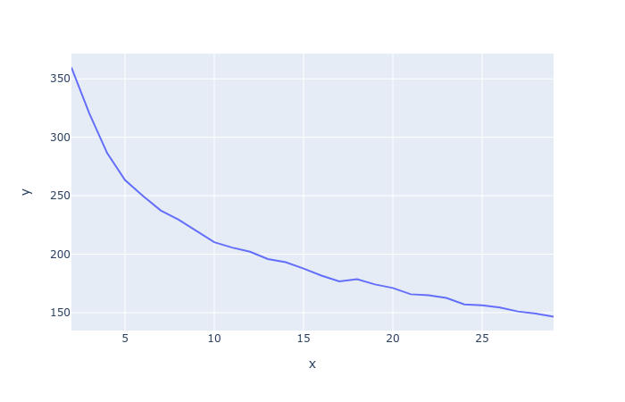
このグラフはこれは各点が自分が所属しているクラスタの中心までの距離の平均を表していて、クラスタ数が多くなれば距離が減りますが、その分粒度が細かくなります。
クラスタ数を増やしても距離があまり減らなくなるところが一般的にいいとされています。
この場合だと５と１０になるでしょうか。

実例で動かすグラフアルゴリズムとグラフデータベース、04_ノードEmbedding：グラフ機械学習へ

Node Embeddingについて

Neo3j Graph Data Science LibraryとNode Embedding

Node Embeddingの算出

検証

3d

4d

10d

クラスタ数について