例題(2):単純な折れ線グラフ
例題(1)ではとりあえずmatplotlibでグラフを作っただけだった.
しかし,これではExcelの方がまだマシなレベルで,使い物にならない.
次の例題はまともなグラフの例である.ここから一気にサンプルコードが長くなる.
import numpy as np # numpy
import matplotlib.pyplot as plt # matplotlib plt
import matplotlib.ticker as ticker # matplotlib ticker
def main():
'''main program'''
# setting
f_out = 'graph02_example.png' # output file (figure)
# data
x = np.arange(0, 5, 0.1)
y1 = np.exp(-x) * np.cos(2*np.pi*x)
y2 = np.exp(-x)
data = {'p1': [x, y1], # data packing
'p2': [x, y2]}
# plot graph
run_plot(f_out, data)
def run_plot(f_out, data):
'''plot graph
[input]
f_out: output file name
data: data for plotting
'''
# (0) setting of matplotlib
# graph
gx = 10 # graph size of x [cm]
gy = 6 # graph size of y [cm]
dpi = 200 # graph DPI (100~600程度)
# font
f_family = 'IPApGothic' # font (sans-serif, serif, IPApGothic)
font_ax = {'size': 10, 'color': 'k'} # 軸ラベルのフォント
fs_le = 9 # 凡例のフォントサイズ
fs_ma = 9 # 主目盛りのフォントサイズ
font_tx = {'size': 10} # テキストのフォント
# 軸ラベル
x_label = 'X' # x軸ラベル
y_label = 'Y' # y軸ラベル
# 軸範囲
x_s = 0 # x軸の最小値
x_e = 5 # x軸の最大値
y_s = -1 # y軸の最小値
y_e = 1 # y軸の最大値
# 目盛り
x_ma = 1 # x軸の主目盛り間隔
x_mi = 0.2 # x軸の副目盛り間隔
y_ma = 0.5 # y軸の主目盛り間隔
y_mi = 0.1 # y軸の副目盛り間隔
# (A) Figure
# (A.1) Font or default parameter
# https://matplotlib.org/stable/api/matplotlib_configuration_api.html
plt.rcParams['font.family'] = f_family
# (A.2) Figureの作成
# https://matplotlib.org/stable/api/_as_gen/matplotlib.pyplot.figure.html
# [Returns]
# Figureオブジェクトが返される。
# [Parameter]
# figsize=(6.4,4.8): グラフサイズ(x,y), 1[cm]=1/2.54[in]
# dpi=100: 出力DPI
tl = False # Figureのスペース自動調整
fc = 'w' # Figureの背景色
ec = None # 枠線の色
lw = None # 枠線の幅
fig = plt.figure(figsize=(gx/2.54, gy/2.54), dpi=dpi,
tight_layout=tl, facecolor=fc, edgecolor=ec,
linewidth=lw)
# (A.3) グラフ間隔の調整(pltまたはfig)
# bottom等はfigure()でtigit_layout=Trueにすれば不要
# https://matplotlib.org/stable/api/_as_gen/matplotlib.pyplot.subplots_adjust.html
bottom = 0.18 # グラフ下側の位置(0~1)
top = 0.95 # グラフ上側の位置(0~1)
left = 0.16 # グラフ左側の位置(0~1)
right = 0.95 # グラフ右側の位置(0~1)
hspace = 0.2 # グラフ(Axes)間の上下余白
wspace = 0.2 # グラフ(Axes)間の左右余白
fig.subplots_adjust(bottom=bottom, top=top, left=left, right=right,
hspace=hspace, wspace=wspace)
# (B) Axes
# (B.1) Axesの追加
# 複数のグラフをタイル状に作成することができる。
# 複数グラフの配置を細かく設定する場合はadd_axes()やadd_gridspec()。
# https://matplotlib.org/stable/api/figure_api.html
# [Returns]
# Axesオブジェクトが返される。
# [Parameter]
# *args=(1,1,1): 行番号,列番号,インデックス
# 1つのFigureに複数のAxesを作る場合に指定する。
# add_subplot(2,1,1): 2行のAxesを作り、その1番目(上側)
# add_subplot(211): 2,1,1と同じだが、簡略記法
# projection='rectilinear': グラフの投影法(polarなど)
# sharex: x軸を共有する際に、共有元のAxisを指定する。
# sharey: sharexのy軸版
# label: Axesに対する凡例名(通常は使わない)
n_row = 1 # 全グラフの行数
n_col = 1 # 全グラフの列数
n_ind = 1 # グラフ番号
fc = 'w' # Axesの背景色(通常は白)
ax = fig.add_subplot(n_row, n_col, n_ind, fc=fc)
# (B.2) 軸ラベル(axis label)の設定
# https://matplotlib.org/stable/api/_as_gen/matplotlib.axes.Axes.set_xlabel.html
# [Parameter]
# xlabel: 軸ラベル
# loc='center': 軸ラベル位置(x: left,center,right; y:bottom,center,top)
# labelpad: 軸ラベルと軸間の余白
# fonddict: 軸ラベルのText設定
ax.set_xlabel(x_label, fontdict=font_ax) # x軸ラベルの設定
ax.set_ylabel(y_label, fontdict=font_ax) # y軸ラベルの設定
# (B.3) 軸の種類の設定
# https://matplotlib.org/stable/api/_as_gen/matplotlib.axes.Axes.set_xscale.html
xscale = 'linear' # x軸の種類(linear, log, symlog, logit)
yscale = 'linear' # y軸の種類(linear, log, symlog, logit)
ax.set_xscale(xscale) # x軸の種類
ax.set_yscale(yscale) # y軸の種類
# (B.4) 軸の範囲の設定
# 自動で設定する場合は、auto=Trueのみにする
# https://matplotlib.org/stable/api/_as_gen/matplotlib.axes.Axes.set_xlim.html
ax.set_xlim(x_s, x_e, auto=False) # x軸の範囲
ax.set_ylim(y_s, y_e, auto=False) # y軸の範囲
# (B.5) 軸のアスペクト比
# x軸とy軸の比率を強制的に設定する場合に行う。
# https://matplotlib.org/stable/api/_as_gen/matplotlib.axes.Axes.set_aspect.html
# https://matplotlib.org/stable/api/_as_gen/matplotlib.axes.Axes.set_box_aspect.html
asp_a = 'auto' # auto:自動, [数値]:x,yの比率
asp_b = None # None:自動, [数値]:x,yのグラフ長さの比率
ax.set_aspect(asp_a) # X軸とY軸の比率を設定する
ax.set_box_aspect(asp_b) # X軸とY軸のグラフ長さの比率を設定する
# (B.6) 目盛り関係の設定
# (B.6.1)主目盛りの位置(Locator)
# https://matplotlib.org/stable/api/ticker_api.html
mal_x = ticker.MultipleLocator(x_ma) # 等間隔目盛り
# mal_x = ticker.IndexLocator(x_ma, x_off) # 等間隔目盛り(+offset)
# mal_x = ticker.LogLocator(base=10) # 対数目盛り
# mal_x = ticker.AutoLocator() # 自動目盛り
# mal_x = ticker.NullLocator() # 目盛りなし
# mal_x = ticker.LinearLocator(nx_ma) # 個数指定目盛り
# mal_x = ticker.FixedLocator([0, 1, 3]) # 位置指定目盛り
mal_y = ticker.MultipleLocator(y_ma) # 等間隔目盛り
# mal_y = ticker.IndexLocator(y_ma, y_off) # 等間隔目盛り(+offset)
# mal_y = ticker.LogLocator(base=10) # 対数目盛り
# mal_y = ticker.AutoLocator() # 自動目盛り
# mal_y = ticker.NullLocator() # 目盛りなし
# mal_y = ticker.LinearLocator(ny_ma) # 個数指定目盛り
# mal_y = ticker.FixedLocator([-1, 0, 1]) # 位置指定目盛り
ax.xaxis.set_major_locator(mal_x) # x軸の主目盛り間隔の設定
ax.yaxis.set_major_locator(mal_y) # y軸の主目盛り間隔の設定
# (B.6.2)主目盛りの表記(Formatter)
# https://matplotlib.org/stable/api/ticker_api.html
maf_x = ticker.ScalarFormatter() # 数値
# maf_x = ticker.NullFormatter() # 目盛り表記なし
# maf_x = ticker.FixedFormatter(['A','B','C','D','E','F']) # 指定表記
# maf_x = ticker.StrMethodFormatter('{x:.1f}m') # format記法
# maf_x = ticker.LogFormatterMathtext(base=10) # log記法(10^x)
maf_y = ticker.ScalarFormatter() # 数値
# maf_y = ticker.NullFormatter() # 目盛り表記なし
# maf_y = ticker.FixedFormatter(['A','B','C','D','E','F']) # 指定表記
# maf_y = ticker.StrMethodFormatter('{x:.1f}m') # format記法
# maf_y = ticker.LogFormatterMathtext(base=10) # log記法(10^x)
ax.xaxis.set_major_formatter(maf_x) # x軸の主目盛り表記の設定
ax.yaxis.set_major_formatter(maf_y) # y軸の主目盛り表記の設定
# (B.6.3) 副目盛りの位置(Locator)
# https://matplotlib.org/stable/api/ticker_api.html
mil_x = ticker.MultipleLocator(x_mi) # 等間隔目盛り
# mil_x = ticker.IndexLocator(x_mi, x_off) # 等間隔目盛り(+offset)
# mil_x = ticker.LogLocator(base=10, subs=np.arange(2, 10)*0.1) # 対数目盛り
# mil_x = ticker.AutoLocator() # 自動目盛り
# mil_x = ticker.NullLocator() # 目盛りなし
# mil_x = ticker.LinearLocator(nx_mi) # 個数指定目盛り
mil_y = ticker.MultipleLocator(y_mi) # 等間隔目盛り
# mil_y = ticker.IndexLocator(y_mi, y_off) # 等間隔目盛り(+offset)
# mil_y = ticker.LogLocator(base=10, subs=np.arange(2, 10)*0.1) # 対数目盛り
# mil_y = ticker.AutoLocator() # 自動目盛り
# mil_y = ticker.NullLocator() # 目盛りなし
# mil_y = ticker.LinearLocator(ny_mi) # 個数指定目盛り
ax.xaxis.set_minor_locator(mil_x) # x軸の副目盛り間隔の設定
ax.yaxis.set_minor_locator(mil_y) # y軸の副目盛り間隔の設定
# (B.6.4) 副目盛りの表記(Formatter)
# https://matplotlib.org/stable/api/ticker_api.html
mif_x = ticker.NullFormatter() # 目盛り表記なし
mif_y = ticker.NullFormatter() # 目盛り表記なし
ax.xaxis.set_minor_formatter(mif_x) # x軸の副目盛り表記の設定
ax.yaxis.set_minor_formatter(mif_y) # y軸の副目盛り表記の設定
# (B.6.5) 目盛り関連の細部の設定
# https://matplotlib.org/stable/api/_as_gen/matplotlib.axes.Axes.tick_params.html
# [Parameter]
# axis: 対象軸(x, y, both)
# which: major, minor, both
# labelsize: フォントサイズ
# top, right, bottom, left: Tickを表記する場所(Trueで表記)
# labeltop: Trueで上側にも目盛りを付ける(labelrightも同様)
# labelrotation: 目盛りの表記角度
# labelcolor: 目盛り表記の色
# pad: 軸と目盛りの間隔
# color: 目盛り線の色
ax.tick_params(axis='both', which='major', labelsize=fs_ma,
top=True, right=True)
ax.tick_params(axis='both', which='minor', top=True, right=True)
# (B.7) グリッドの設定
# https://matplotlib.org/stable/api/_as_gen/matplotlib.axes.Axes.grid.html
gb = False # 出力の有無(Falseかつ、lsなどの指定なしで、出力なし)
which = 'major' # 目盛りの指定(major, minor, both)
axis = 'both' # X,Y軸の指定(x, y, both)
color = 'gray' # 線色
ls = '-' # 線種('-', '--', '-.', ':')
lw = 0.5 # 線幅
ax.grid(b=gb, which=which, axis=axis) # Falseの場合
# ax.grid(b=gb, which=which, axis=axis, c=color, ls=ls, lw=lw)
# (B.8) 直線
# axhline(), axvline(): 横線, 縦線(端から端まで)
# axhspan(), asvspan(): 横線, 縦線(始点と終点指定)
# axline(): 直線
# https://matplotlib.org/stable/api/_as_gen/matplotlib.axes.Axes.axhline.html
# [Parameter]
py = 0 # 横線の位置(y座標)
color = 'k' # 線色
ls = '-' # 線種('-', '--', '-.', ':')
lw = 0.5 # 線幅
ax.axhline(y=py, c=color, ls=ls, lw=lw)
# (C) Plot
# (C.1) plot(): 折れ線グラフ
# 散布図はscatter()
# https://matplotlib.org/stable/api/_as_gen/matplotlib.pyplot.plot.html
# [Returns]
# Line2Dオブジェクト(配列)が返される。
# [Parameter]
# *args: xデータ, yデータ, [fmt]
# x,yデータはx軸とy軸のデータ(リストなど)
# fmtは線や点の簡易的記法による指定
# *kwargs: Line2Dの設定値(多数あり)
d_x = data['p1'][0] # x data(適宜変更)
d_y = data['p1'][1] # y data(適宜変更)
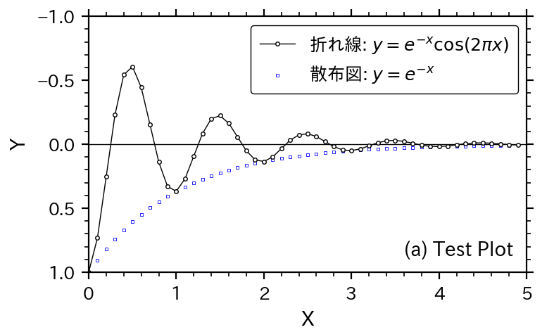
label = r'折れ線: $y = e^{-x} \cos(2 \pi x)$' # 凡例(なしはNone)
ls = '-' # 線種('-', '--', '-.', ':')
lw = 0.5 # 線幅
color = 'k' # 線色(k, r, g, b, etc.)
marker = 'o' # marker(o, s, v, ^, D, +, x, etc.; None=なし)
mec = 'k' # markerの線色(k, r, g, b, etc.)
mew = 0.5 # markerの線幅
mfc = 'w' # markerの色(none, k, r, g, b, w, etc.)
ms = 2 # markerサイズ
markevery = None # markerの出力間隔(None=全部, 2は2個毎)
ax.plot(d_x, d_y, label=label,
ls=ls, lw=lw, c=color, marker=marker,
mec=mec, mew=mew, mfc=mfc, ms=ms,
markevery=markevery)
# (C.2) scatter(): 散布図
# https://matplotlib.org/stable/api/_as_gen/matplotlib.pyplot.scatter.html
# [Returns]
# PathCollectionオブジェクトが返される
# [Parameter]
# x, y: x, yデータ(リストなど)
# その他、scatterの設定値(plotと異なるので注意)
d_x = data['p2'][0] # x data(適宜変更)
d_y = data['p2'][1] # y data(適宜変更)
label = r'散布図: $y = e^{-x}$' # 凡例(なしはNone)
ms = 2 # markerサイズ
mfc = 'w' # markerの色(none, k, r, g, b, w, etc.)
marker = 's' # marker(o, s, v, ^, D, +, x, etc.; None=なし)
mec = 'b' # markerの線色(k, r, g, b, etc.)
mew = 0.3 # markerの線幅
ax.scatter(d_x, d_y, label=label,
s=ms, c=mfc, marker=marker,
linewidths=mew, edgecolors=mec)
# (D) Others: 凡例、テキストなど
# (D.1) 凡例
# (D.1.1) 凡例データの一覧を得る
handles, labels = ax.get_legend_handles_labels()
# (D.1.2) 凡例の作成
# https://matplotlib.org/stable/api/_as_gen/matplotlib.axes.Axes.legend.html
anc = (1, 1) # 凡例の配置場所(0~1の相対位置)
loc = 'upper right' # 配置箇所:upper,center,lower; left,center,right; best
ti = None # 凡例のタイトル(なし=None or '')
ti_fs = 9 # 凡例のタイトルのフォントサイズ
ncol = 1 # 凡例の列数
fc = 'w' # 凡例の背景色(なし=none)
ec = 'k' # 枠線の色(なし=none)
fa = 1.0 # 透明度(0で透明, 1で透明なし)
bp = 0.5 # 凡例の枠の余白(default=0.4)
ms = 1.0 # マーカーの倍率(default=1.0)
sha = False # True:影付き、False:影なし
fb = True # 凡例の角:True:丸、False:四角
bap = 0.5 # 凡例の外側の余白(default=0.5)
ls = 0.5 # 凡例間の上下余白
cs = 2.0 # 凡例間の左右余白
legend = ax.legend(handles, labels, title=ti,
title_fontsize=ti_fs, loc=loc,
bbox_to_anchor=anc, ncol=ncol, facecolor=fc,
edgecolor=ec, framealpha=fa, fontsize=fs_le,
borderpad=bp, shadow=sha, markerscale=ms,
fancybox=fb, labelspacing=ls, columnspacing=cs,
borderaxespad=bap)
# (D.1.3) 凡例の細かい設定
legend.get_frame().set_linestyle('-') # 枠線の種類
legend.get_frame().set_linewidth(0.5) # 枠線の太さ
# (D.2) テキスト
# https://matplotlib.org/stable/api/_as_gen/matplotlib.pyplot.text.html
txt = '(a) Test Plot' # テキスト文字列
px = 0.97 # x位置(transformで基準座標の変更)
py = 0.05 # y位置(transformで基準座標の変更)
tf = ax.transAxes # 基準座標(ax.transAxes, fig.transFigure)
ha = 'right' # 左右位置(left, center, right)
va = 'bottom' # 上下位置(bottom, center, top, baseline)
rot = 0 # 回転角度(左回転)
color = 'k' # テキストの色
ax.text(x=px, y=py, s=txt, font=font_tx, ha=ha, va=va, color=color,
rotation=rot, transform=tf)
# (E) save figure
# https://matplotlib.org/stable/api/_as_gen/matplotlib.pyplot.savefig.html
# [Parameters]
# fname: 出力ファイル名
# dpi: 出力DPI(Figure設定時のdpiが優先)
print(f'write: {f_out}')
plt.savefig(fname=f_out) # save figure
# (F) close
plt.close()
if __name__ == '__main__':
main()
これを実行すると,次のようなグラフが作成される.

注意事項
もし,以下のようなエラーが出た場合は,日本語フォントのインストールがうまくいっていない.もしくは,Linux以外で実行している.
findfont: Font family ['IPApGothic'] not found. Falling back to DejaVu Sans.
この場合,23行目を以下のように変更する.
f_family = 'sans-serif' # font (sans-serif, serif, IPApGothic)
そして,日本語の部分を削除すれば良い.
解説
プログラムの概要
main()
メインプログラム部分.
データ入力やグラフ部分が複雑化する場合があるので,グラフ部分を関数化している.
run_plot()
グラフ作成部分.
run_plot()の引数は出力ファイル名とplotするデータとしている.
長い関数となっているが,以下に示すように,A,B,Cと番号を付けているので,それなりには分かりやすい,はず.
関数をより細かく区分したり,オブジェクト化することも可能だが,使いまわしが良いように単一の関数とした.
(0) setting of matplotlib
グラフの主要なパラメータを明示的に設定している.
これらはグラフに応じて適宜変更される基本的なパラメータである.
ただし,ここでは変数を宣言しただけで,グラフへの設定はまだ実施されていない.
(A) Figure
Figureオブジェクトを作成し,設定する.
この部分は下記で詳細を述べる.
(B) Axes
Axes(グラフ枠)の設定だが,これが非常に大変で,matplotlibの山場の一つである.
(C) Plot
データをプロットする.例題では,折れ線グラフ(plot)と散布図(scatter)を使っている.
(D) Others: 凡例,テキストなど
凡例や,テキスト挿入などを行う.
(E) save figure
グラフを出力する.
(F) close
作成したFigureを閉じて終了.
(A) Figure
Figureオブジェクトを作成する.
(A.1) Font or default parameter
    # (A.1) Font or default parameter
    # https://matplotlib.org/stable/api/matplotlib_configuration_api.html
    plt.rcParams['font.family'] = f_family
(A.1)で,図全体に関わるデフォルト値を変更する.
rcParamsは非常に多くのパラメータがあるけれども,フォントの種類のみで良い.
軸ラベルや目盛りのフォントの種類はグラフ全体で統一するのが普通である.
plt.rcParams['font.family'] = f_family
はグラフの基本のフォント種類を一括して設定している.
フォントサイズについては,それぞれ個別に設定する.
(A.2) Figure
(A.2)でFigureオブジェクトを作成する.
    # (A.2) Figureの作成
    # https://matplotlib.org/stable/api/_as_gen/matplotlib.pyplot.figure.html
    # [Returns]
    #   Figureオブジェクトが返される.
    # [Parameter]
    # figsize=(6.4,4.8): グラフサイズ(x,y), 1[cm]=1/2.54[in]
    # dpi=100: 出力DPI
    tl = False                  # Figureのスペース自動調整
    fc = 'w'                    # Figureの背景色
    ec = None                   # 枠線の色
    lw = None                   # 枠線の幅
    fig = plt.figure(figsize=(gx/2.54, gy/2.54), dpi=dpi,
                     tight_layout=tl, facecolor=fc, edgecolor=ec,
                     linewidth=lw)
maptlotlibはオブジェクト指向だが,オブジェクトの設定を,作成時に設定するものと,作成後に設定するものと,2種類ある.
Figureは作成時に設定するパターンである.
そのため,多数のパラメータを一気に設定することになるが,そういうものだと割り切ってほしい.
(A.2)ではグラフサイズと出力ファイルの解像度を設定する.
背景色なども設定できるが,通常は白(w=whiteの略)を使う.
(A.3) グラフ間隔の調整
(A.3)はグラフの余白を設定する.
    # (A.3) グラフ間隔の調整(pltまたはfig)
    # bottom等はfigure()でtigit_layout=Trueにすれば不要
    # https://matplotlib.org/stable/api/_as_gen/matplotlib.pyplot.subplots_adjust.html
    bottom = 0.18                # グラフ下側の位置(0~1)
    top = 0.95                  # グラフ上側の位置(0~1)
    left = 0.16                 # グラフ左側の位置(0~1)
    right = 0.95                # グラフ右側の位置(0~1)
    hspace = 0.2                # グラフ(Axes)間の上下余白
    wspace = 0.2                # グラフ(Axes)間の左右余白
    fig.subplots_adjust(bottom=bottom, top=top, left=left, right=right,
                        hspace=hspace, wspace=wspace)
Figureは図面全体だが,1つの図面に複数のグラフをプロットすることができる.
hspace, wspaceは複数グラフ間の余白の設定である.今のところは,1つのグラフだけなので,関係ない.
演習
サンプルコードを基に,下記の演習問題に解答せよ.
解答はコメント欄参照.
演習(1):軸の範囲と目盛りの簡易調整
下図のように,X軸とY軸の範囲と目盛りを変更せよ.
x軸は,範囲が0~3,目盛りが0.5と0.1.y軸は,範囲が-1.2~1.2,目盛りが0.4と0.1.

演習(2):軸の反転
下図のように,Y軸を反転させよ.
演習(3):図の大きさ調整,余白調整
下図のように,図の大きさを横12cm×縦5cmとし,余白をうまく調整せよ.※X軸,Y軸の設定は例題のまま.

次の記事
例題演習matplotlib(3):Axes(軸)の設定
https://qiita.com/s4s/items/99c8c6aad1339dfbc544