matlab関数フィッティング (正弦波フィット)

optimization toolbox でも フィッティングができる．
今回はlsqnonlinを使う．

まずフィッティングするデータを用意する．

x = pi*(0:30:360)/180;
y = 2*rand(1)*sin(x-randn(1)*pi+pi/2)+0.2;
yraw = y+0.17*randn(size(x)); % 正規乱数を足す．このデータにフィッティングする．

関数ハンドルを用意してフィッティングする．パラメータは位相，ベースラインと波の大きさ．

sinfunc = @(v, x) (v(1)*sin(x-v(2))+v(3)); % 関数ハンドル

%フィッテイングの際の初期値
vinit(1) = max(y)+mean(y);
vinit(2) = 0;
vinit(3) = max(y);

% フィッティングアルゴリズムなどのオプション
options = optimoptions('lsqnonlin', 'MaxIter', 10000,...
	'Algorithm', 'trust-region-reflective', 'Tolx', 10^-15, 'TolFun', 10^-15,...
	'ScaleProblem', 'none', 'MaxFunEvals', length(x)*200, 'Display', 'off');

% 変数の上限と下限
ub = [vinit(1)*2, 2*pi, vinit(1)];
lb = [0, 0, min(y)];
	
% 最適化する関数
efunc = @(v) abs((sinfunc(v,x) - y));

% 正弦波フィットの場合は位相の初期値を色々試す方が良い 
% (y の最大値をから初期値をもとめても良い)
initphz = [0:30:360]*pi/180;
for i = 1:length(initphz)
	vinit(2) = initphz(i);
	[params{i}, f(i), flag{i}, lamb{i}] = ...
      lsqnonlin(efunc, vinit, lb, ub,options);	
end
[~, o] = min(f); 
optparam = params{o};

プロットしてみる．

figure; hold on
xopt = 0:0.1:2*pi;
plot(x,yraw,'d')
plot(xopt, sinfunc(optparam, xopt), 'k-')
plot(x, y, 'r-ーo')

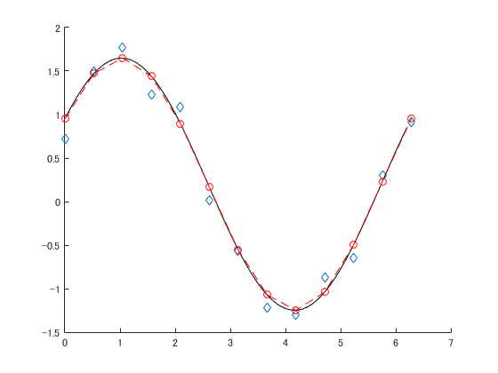
青がフィッティングに使ったデータで赤丸がノイズを足す前．黒線はフィッティングの結果である．
良い感じ．

基本的な流れは，

• フィッティングに使う関数を用意
• 初期値と上限値を考える
• 初期値が難しい場所は色々値を変えてみる
• 一番良かったパラメータを採用

である．

パラメータが多かったり初期値がまずいと収束に時間がかかるので parfor なんかを使ったほうが良い．