Word2vecの簡易版を眺めてみる - TensorFlowチュートリアル

TensorFlowのチュートリアルVector Representations of Words(日本語訳)に記載されていtensorflow/examples/tutorials/word2vec/word2vec_basic.pyについて詳細を見ていくことでWord2vecがやっていることを理解していきます。

Word2vecの概要

この本を読んでもらえると大枠は掴めると思います！

word2vecによる自然言語処理

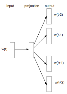
Skip-gram

簡単に言ってしまうと、図1のようにある1単語から複数の単語を予測するというモデルになります。

図 1

word2vec_basic.py

word2vec_basic.pyには大きく分けて6つのStepが記述されています。

Step 1: Download the data.

http://mattmahoney.net/dc/text8.zipからデータをダウンロード
ダウンロードしたzipファイルから中身を取り出し、バイト列を文字列に変換
- f.namelist()[0]はファイル名
- tf.compat.as_strで文字列に変換
空白文字列で単語を分割し配列にする

step1

with zipfile.ZipFile(filename) as f:
    data = tf.compat.as_str(f.read(f.namelist()[0])).split()

Step 2: Build the dictionary and replace rare words with UNK token.

ここでは大きく分けて3つの処理がされています。

各単語の出現数をカウントする
辞書(dictionary)の作成
- 辞書に登録されている単語が指定した数以上になった場合UNKというシンボルに変換する
- UNK + 単語数　= 50000
  - 単語の数え上げ
    - collections.Counter(words)
    - この時に出現回数が多い単語順になる
  - 出現が多い順に上位49999を取り出す
    - collections.Counter(words).most_common(vocabulary_size - 1)
  - UNKシンボルのものと含めて指定した50000にする
    - count.extend(・・・) # count = [['UNK', -1]]
- indexをキーとし、valueを単語としたDictionaryを作る
  - dict(zip(dictionary.values(), dictionary.keys()))
辞書で定義したindexで文章全体を置き換える

step2

vocabulary_size = 50000 # 取り扱う単語数(`vocabulary_size`)を50000とする
def build_dataset(words):
  count = [['UNK', -1]]
  count.extend(collections.Counter(words).most_common(vocabulary_size - 1))
  dictionary = dict()
  for word, _ in count:
    dictionary[word] = len(dictionary)
  data = list()
  unk_count = 0
  for word in words:
    if word in dictionary:
      index = dictionary[word]
    else:
      index = 0  # dictionary['UNK']
      unk_count += 1
    data.append(index)
  count[0][1] = unk_count
  reverse_dictionary = dict(zip(dictionary.values(), dictionary.keys()))
  return data, count, dictionary, reverse_dictionary

Step 3: Function to generate a training batch for the skip-gram model.

1回の学習で使用するターゲット単語とその正解ペアを生成する

関数`generate_batch`引数について

skip_window
- skip-gramモデル(図1参照)は、ターゲットの単語から周辺単語を予測するために、skip_windowで周辺の単語の範囲を指定する。
  - 例: 5を指定した場合、ターゲットとなる単語の前後5単語、合計11個の単語を取り扱う
num_skips
- skip_windowで指定した単語の中でターゲットとなる単語以外のものから、ターゲットの単語から予測される正解の単語(label)を何文字取得するかnum_skipsで指定する
batch_size
- 1回の学習で使用するターゲット単語とその正解ペアの数を指定する

step3

data_index = 0
def generate_batch(batch_size, num_skips, skip_window):
  global data_index
  assert batch_size % num_skips == 0
  assert num_skips <= 2 * skip_window
  batch = np.ndarray(shape=(batch_size), dtype=np.int32)
  labels = np.ndarray(shape=(batch_size, 1), dtype=np.int32)
  span = 2 * skip_window + 1 # [ skip_window target skip_window ]
  buffer = collections.deque(maxlen=span)
  for _ in range(span):
    buffer.append(data[data_index])
    data_index = (data_index + 1) % len(data)
  for i in range(batch_size // num_skips):
    target = skip_window  # target label at the center of the buffer
    targets_to_avoid = [ skip_window ]
    for j in range(num_skips):
      while target in targets_to_avoid:
        target = random.randint(0, span - 1)
      targets_to_avoid.append(target)
      batch[i * num_skips + j] = buffer[skip_window]
      labels[i * num_skips + j, 0] = buffer[target]
    buffer.append(data[data_index])
    data_index = (data_index + 1) % len(data)
  return batch, labels

Step 4: Build and train a skip-gram model.

Step2で辞書を作成し、文章を整数で表すことができました。
またStep3の関数を用いて学習に使用するデータを取得できますが、整数であるため、各単語を特徴を表すベクトルに変換する必要があります。

そこで、TensorFlowでは便利なヘルパーtf.nn.embedding_lookupが用意されており、これを使用して各単語をベクトルに変換します。

実装上は一様分布の-1.0〜1.0の範囲から乱数を出力しそれを初期値としています。

    embeddings = tf.Variable(
        tf.random_uniform([vocabulary_size, embedding_size], -1.0, 1.0))
    embed = tf.nn.embedding_lookup(embeddings, train_inputs)

目的関数にはNoise Contrastive Estimation (NCE)関数(tf.nn.nce_loss)を用い、勾配降下法でパラメーターを修正していきます。

    # Construct the variables for the NCE loss
    nce_weights = tf.Variable(
        tf.truncated_normal([vocabulary_size, embedding_size],
                            stddev=1.0 / math.sqrt(embedding_size)))
    nce_biases = tf.Variable(tf.zeros([vocabulary_size]))

  # Compute the average NCE loss for the batch.
  # tf.nce_loss automatically draws a new sample of the negative labels each
  # time we evaluate the loss.
  loss = tf.reduce_mean(
      tf.nn.nce_loss(nce_weights, nce_biases, embed, train_labels,
                     num_sampled, vocabulary_size))

  # Construct the SGD optimizer using a learning rate of 1.0.
  optimizer = tf.train.GradientDescentOptimizer(1.0).minimize(loss)

step4

batch_size = 128
embedding_size = 128  # Dimension of the embedding vector.
skip_window = 1       # How many words to consider left and right.
num_skips = 2         # How many times to reuse an input to generate a label.

# We pick a random validation set to sample nearest neighbors. Here we limit the
# validation samples to the words that have a low numeric ID, which by
# construction are also the most frequent.
valid_size = 16     # Random set of words to evaluate similarity on.
valid_window = 100  # Only pick dev samples in the head of the distribution.
valid_examples = np.random.choice(valid_window, valid_size, replace=False)
num_sampled = 64    # Number of negative examples to sample.

graph = tf.Graph()

with graph.as_default():

  # Input data.
  train_inputs = tf.placeholder(tf.int32, shape=[batch_size])
  train_labels = tf.placeholder(tf.int32, shape=[batch_size, 1])
  valid_dataset = tf.constant(valid_examples, dtype=tf.int32)

  # Ops and variables pinned to the CPU because of missing GPU implementation
  with tf.device('/cpu:0'):
    # Look up embeddings for inputs.
    embeddings = tf.Variable(
        tf.random_uniform([vocabulary_size, embedding_size], -1.0, 1.0))
    embed = tf.nn.embedding_lookup(embeddings, train_inputs)

    # Construct the variables for the NCE loss
    nce_weights = tf.Variable(
        tf.truncated_normal([vocabulary_size, embedding_size],
                            stddev=1.0 / math.sqrt(embedding_size)))
    nce_biases = tf.Variable(tf.zeros([vocabulary_size]))

  # Compute the average NCE loss for the batch.
  # tf.nce_loss automatically draws a new sample of the negative labels each
  # time we evaluate the loss.
  loss = tf.reduce_mean(
      tf.nn.nce_loss(nce_weights, nce_biases, embed, train_labels,
                     num_sampled, vocabulary_size))

  # Construct the SGD optimizer using a learning rate of 1.0.
  optimizer = tf.train.GradientDescentOptimizer(1.0).minimize(loss)

  # Compute the cosine similarity between minibatch examples and all embeddings.
  norm = tf.sqrt(tf.reduce_sum(tf.square(embeddings), 1, keep_dims=True))
  normalized_embeddings = embeddings / norm
  valid_embeddings = tf.nn.embedding_lookup(
      normalized_embeddings, valid_dataset)
  similarity = tf.matmul(
      valid_embeddings, normalized_embeddings, transpose_b=True)

  # Add variable initializer.
  init = tf.initialize_all_variables()

Step 5: Begin training.

ログを出力してる部分など一部省略しているのでコピペしても動きません！

step5

num_steps = 100001

with tf.Session(graph=graph) as session:
  init.run()

  for step in xrange(num_steps):
    batch_inputs, batch_labels = generate_batch(
        batch_size, num_skips, skip_window)
    feed_dict = {train_inputs : batch_inputs, train_labels : batch_labels}

    # We perform one update step by evaluating the optimizer op (including it
    # in the list of returned values for session.run()
    _, loss_val = session.run([optimizer, loss], feed_dict=feed_dict)

  # グラフ描画用
  final_embeddings = normalized_embeddings.eval()

Step 6: Visualize the embeddings.

ここでは結果を可視化しているだけなので省略

まとめ

このmodelで学習時に変更されるパラメータが

nce_weights
nce_biases

はいつも通りでわかったのですが、最終的にグラフを描く時にembeddingsを各単語の特徴ベクトルとして扱っているのを見ると

embeddings

も学習時に更新されているように思います、実際session.run([optimizer, loss], feed_dict=feed_dict)の実行前後でembeddingsの値が変わっていました。

Noise-contrastive estmiation（tf.nn.nce_loss）を理解しないとなぁ。

どなたかembeddingsが更新されるロジックご存知の方おられましたら、教えて下さい！

Word2vecの簡易版を眺めてみる - TensorFlowチュートリアル

Word2vecの簡易版を眺めてみる - TensorFlowチュートリアル

Word2vecの概要

Skip-gram

word2vec_basic.py

Step 1: Download the data.

Step 2: Build the dictionary and replace rare words with UNK token.

Step 3: Function to generate a training batch for the skip-gram model.

関数generate_batch引数について

Step 4: Build and train a skip-gram model.

Step 5: Begin training.

Step 6: Visualize the embeddings.

まとめ

参考

関数`generate_batch`引数について