1. FET の非線形性(艶っぽい・偶数倍音)
■ JFET の Id–Vgs 特性(ソフトクリッピングの源)
JFET のドレイン電流は近似的に
Id = Idss * (1 - Vgs / Vp)^2 (Vgs < 0)
・Id–Vgs が 放物線(2次曲線)
・入力を大きくすると 緩やかに飽和
→ クリッピングが 滑らか・非対称 になりやすい
この「放物線の2次非線形」は、テイラー展開すると偶数項が残るため、
偶数倍音(2f, 4f)が強調
■ MOSFET(オーバードライブ)
MOSFET の Id–Vgs(飽和領域)は
Id ≈ (1/2) * k * (Vgs - Vth)^2
・こちらも 2次非線形(Even-order)
・波形の上側だけが先につぶれる(非対称クリップ)
結果:
→ 偶数倍音が強く、温かい・艶っぽい音色になる
2. BJT の非線形性(攻撃的・奇数倍音)
■ BJT の Ic–Vbe 特性
BJT の基本式:
Ic = Is * exp(Vbe / Vt)
この指数関数は 奇数項主体の急峻非線形 を作る。
指数関数をテイラー展開すると
exp(x) = 1 + x + x^2/2! + x^3/3! + …
ただし実際の回路では バイアス点の前後対称 になりやすく、
クリッピングが上下ほぼ対称 → 偶数次が相殺される。
結果:
奇数倍音(3f, 5f, 7f)が支配的
→ エッジが立つ・ロック向きの攻撃的サウンドになる
3. クリッピング形状と倍音(式による説明)
■ 波形の対称性と倍音
入力波形を x(t) とし、
非線形関数 f(x) に通した出力を y(t) とする。
y(t) = f( x(t) )
ここで f(x) が
● 偶関数(f(-x)=f(x))
→ 偶数次倍音が強い(FET系、非対称クリップ)
● 奇関数(f(-x)=-f(x))
→ 奇数次倍音が強い(BJT系、対称クリップ)
FET の Id–Vgs(2次曲線)は 偶関数成分 が多く、
BJT の指数特性は回路全体として 奇関数に近くなる。
4. 実際のFFTを式で表した場合
入力を正弦波とする:
x(t) = A * sin(2πft)
非線形を「ソフトクリップ(FET)」で近似すると:
y(t) = a1 * sin(2πf t)
      + a2 * sin(4πf t)
      + a3 * sin(6πf t) + …
偶数倍音(2f, 4f, 6f)が強い。
非線形を「ハードクリップ(BJT)」で近似すると:
y(t) ≈ b1 * sin(2πf t)
      + b3 * sin(6πf t)
      + b5 * sin(10πf t) + …
奇数倍音(3f, 5f, 7f)の比率が高い。
5. 回路例(式ベース)
■ FETソフトクリップ系(MOSFET OD)
Vin → Gate
Drain → Load R
Source → GND(もしくは小抵抗)
クリップ電圧:
Vclip ≈ Vth + sqrt( 2*Id / k )
非対称クリップが偶数倍音の源。
■ BJTディストーション系(Rangemaster)
Ic ≈ Is * exp(Vbe / Vt)
Vout = Vcc - Ic * Rc
Vbe の急峻性によりクリップが正負対称 → 奇数倍音。
6. 音色に関する技術的結論
FET:二乗特性 → 非対称 → 偶数倍音 → 艶・甘さ・チューブ感
BJT:指数特性 → 対称 → 奇数倍音 → エッジ・攻撃性・ロック
この式レベルの違いが、
「艶っぽいFET」「ストレートバイポーラ」
というギター用語的な音の差を数学的に説明する。
仕様
・Google Colab / Jupyter で動作
・matplotlib の色指定禁止(自動色)
・純正Python+numpy+matplotlibのみ
・FET=2次非線形、BJT=対称クリップの簡易モデル
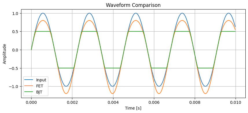
・波形表示(Time domain)
・FFT(Magnitude spectrum)を表示
・タイトル/軸ラベル/凡例は英語
Python Code(matplotlibで波形&FFTプロット)
# ===========================================
# Program: fet_bjt_harmonics_fft.py
# Overview: Compare FET (even-order) vs BJT (odd-order) distortion
# Usage: Run in Google Colab or Jupyter
# ===========================================
import numpy as np
import matplotlib.pyplot as plt
# ================
# Parameters
# ================
fs = 48000 # Sampling frequency
f0 = 440 # Input sine frequency (A4)
duration = 0.01 # Short window for viewing waveform
t = np.linspace(0, duration, int(fs*duration), endpoint=False)
A = 1.0 # Input amplitude
# ======================================================
# Nonlinear models (simple representation)
# ======================================================
# 1) FET-like soft clipping (quadratic nonlinearity)
def fet_soft_clip(x):
return x - 0.2 * x**2 # even-order distortion
# 2) BJT-like symmetric hard clipping
def bjt_hard_clip(x):
limit = 0.5
return np.clip(x, -limit, limit) # odd-order dominant
# ================
# Generate signals
# ================
x = A * np.sin(2*np.pi*f0*t)
y_fet = fet_soft_clip(x)
y_bjt = bjt_hard_clip(x)
# ================
# FFT Function
# ================
def compute_fft(sig, fs):
N = len(sig)
freqs = np.fft.rfftfreq(N, 1/fs)
fft_mag = np.abs(np.fft.rfft(sig)) / N
return freqs, fft_mag
freq_fet, mag_fet = compute_fft(y_fet, fs)
freq_bjt, mag_bjt = compute_fft(y_bjt, fs)
# ===========================
# Time domain: plotting
# ===========================
plt.figure(figsize=(10, 4))
plt.plot(t[:1000], x[:1000], label="Input")
plt.plot(t[:1000], y_fet[:1000], label="FET")
plt.plot(t[:1000], y_bjt[:1000], label="BJT")
plt.title("Waveform Comparison")
plt.xlabel("Time [s]")
plt.ylabel("Amplitude")
plt.legend()
plt.grid(True)
plt.show()
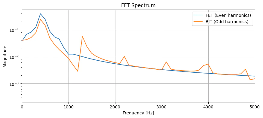
# ===========================
# FFT: plotting
# ===========================
plt.figure(figsize=(10, 4))
plt.semilogy(freq_fet, mag_fet, label="FET (Even harmonics)")
plt.semilogy(freq_bjt, mag_bjt, label="BJT (Odd harmonics)")
plt.xlim(0, 5000)
plt.title("FFT Spectrum")
plt.xlabel("Frequency [Hz]")
plt.ylabel("Magnitude")
plt.legend()
plt.grid(True)
plt.show()
コードの仕組み(技術解説)
● FET(偶数倍音)
return x - 0.2 * x**2
2次項(x²)が「偶関数」→ 偶数倍音(2f, 4f, …)が生成。
● BJT(奇数倍音)
np.clip(x, -limit, limit)
対称クリッピング → 奇関数成分 → 奇数倍音(3f, 5f, 7f)優位。
● FFT解析
fft = abs(FFT(sig)) / N
soft / hard clipping の違いがそのまま倍音スペクトルに現れる。