深層学習

#Day1

入力層ー中間層

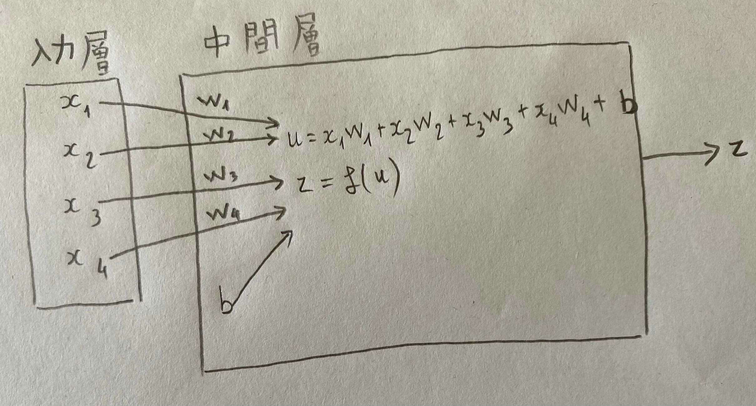
x_i：入力\\
w_i：重み\\
b：バイアス\\
f：活性化関数\\
z：出力\\

配列式

\boldsymbol{W} = \begin{pmatrix} w_{1} \\ w_{2} \\ \vdots \\ w_{n} \end{pmatrix} \qquad \boldsymbol{x} = \begin{pmatrix} x_{1} \\ x_{2} \\ \vdots \\ x_{n} \end{pmatrix}\\
u = w_{1}x_{1} + w_{2}x_{2} +\dots + w_{n}x_{n} + b\\
u = \boldsymbol{W}\boldsymbol{x} + b

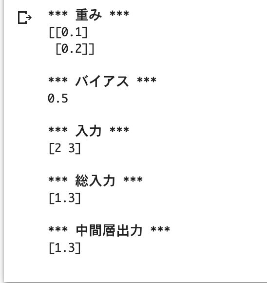
コード

W = np.array([[0.1], [0.2]])
b = 0.5
x = np.array([2, 3])
u = np.dot(x, W) + b
z = functions.relu(u)

考察

重回帰分析と似ている。
異なるのが、活性化関数の導入

活性化関数

次の層への出力の大きさ・信号ON/OFFを決める非線形関数（関数の図が直線でない）

使い分け

中間層用

• ReLU関数（主流）
• Sigmoidシグモイド関数
• Step ステップ関数

出力層用

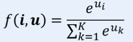
• Softmaxソフトマックス関数（クラス分類２つ以上の場合）
• Sigmoidシグモイド関数
• 恒等写像関数（f(x) = x)

Step ステップ関数

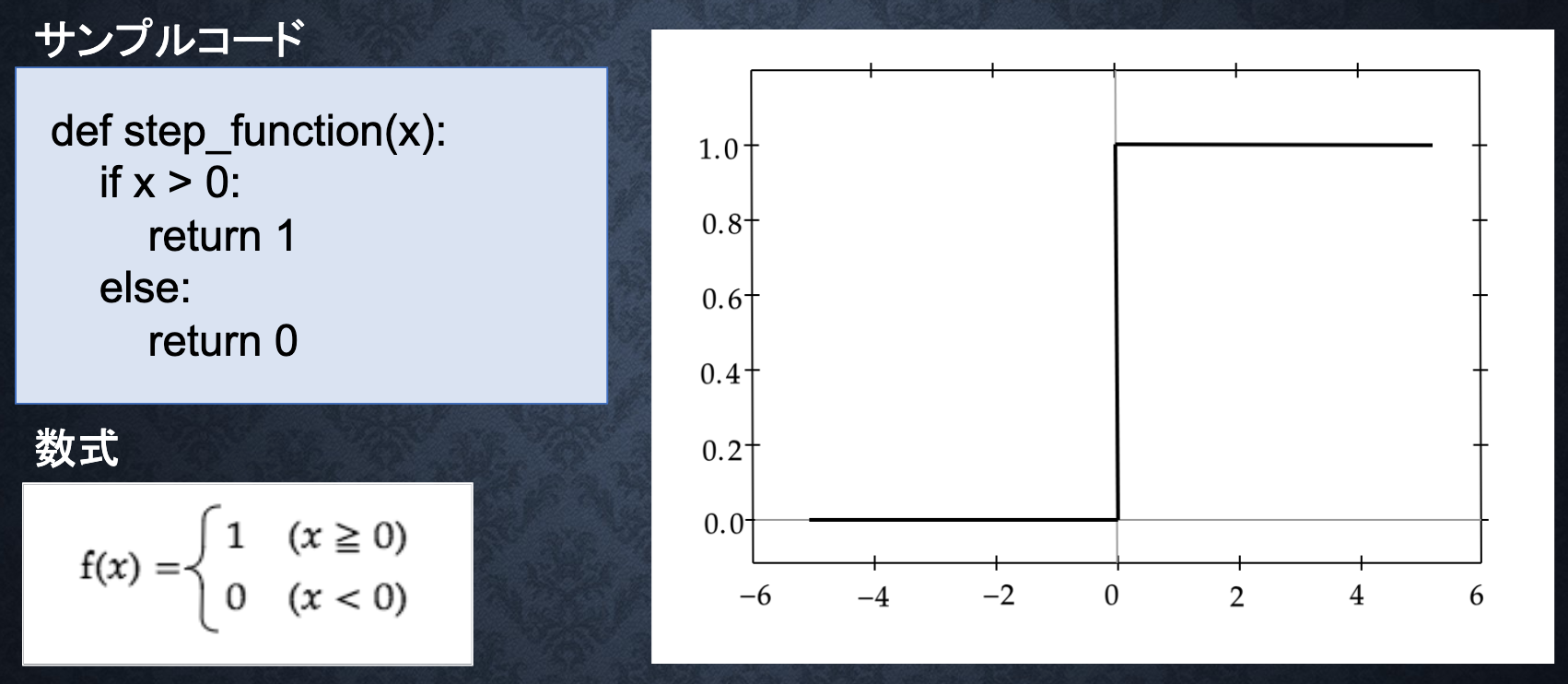
パーセプトロンで利用される関数
課題：０〜１表現できず、線形分離可能なものしか学習できない

Sigmoidシグモイド関数

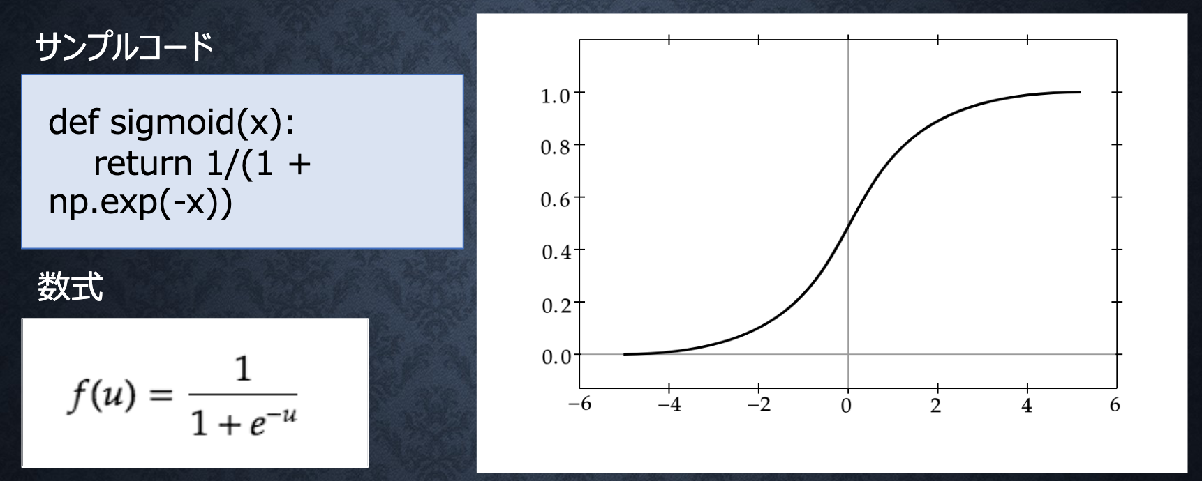
ON/OFFしかできないステップ関数に対し、信号の強弱を調整できる関数
課題：大きな値では出力が微小のため、勾配消失問題が落ちやすい

ReLU関数

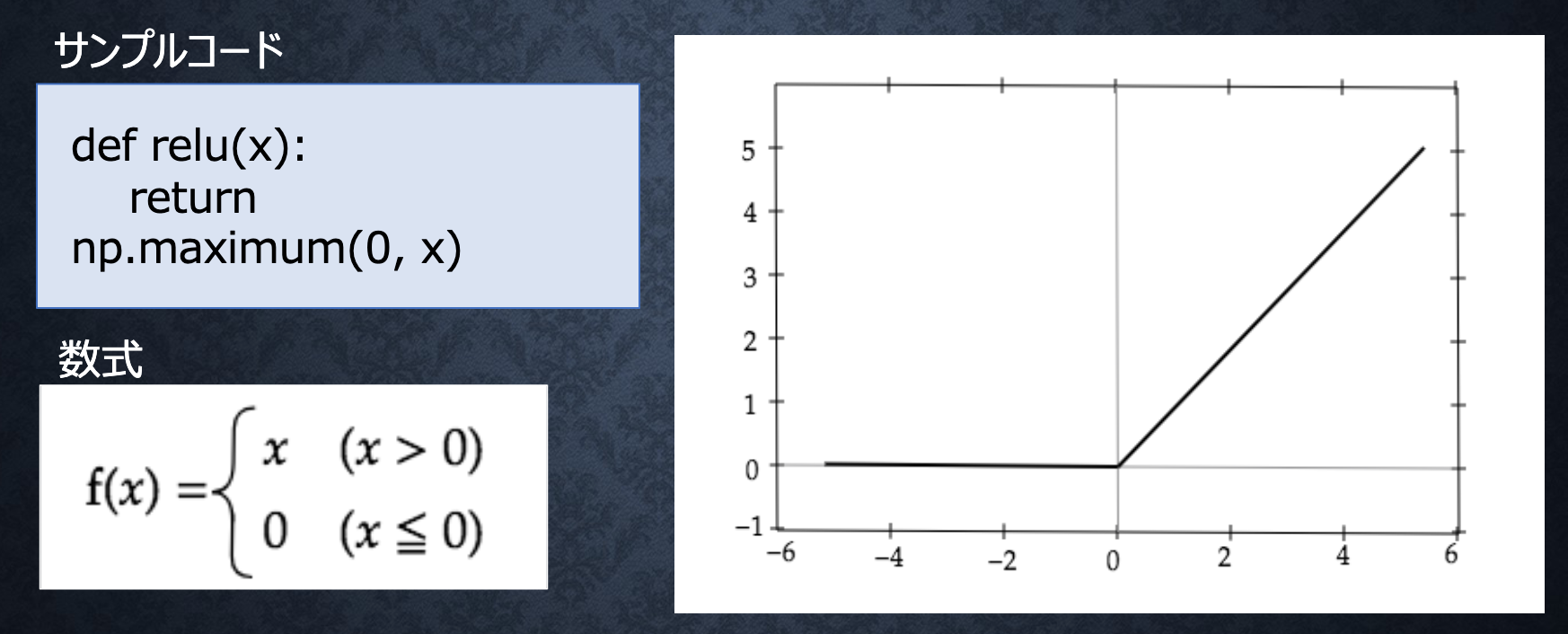
勾配消失問題を回避、スパース化（影響が少ない重みを0に）を貢献

Softmaxソフトマックス関数

コード

def softmax(x):
    if x.ndim == 2:
        x = x.T
        x = x - np.max(x, axis=0)
        y = np.exp(x) / np.sum(np.exp(x), axis=0)
        return y.T

    x = x - np.max(x) # オーバーフロー対策
    return np.exp(x) / np.sum(np.exp(x))

出力層

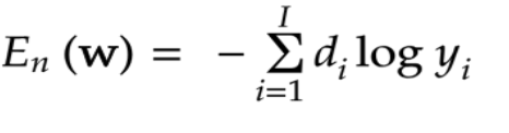
誤差関数

出力層のアウトプット（d）とラベル（y）の間、どのぐらい差があるか計算する関数

####二乗誤差

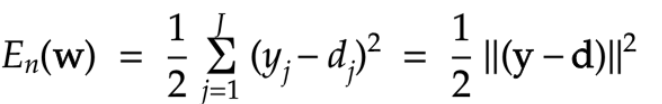
※1/2あるのは、微分する際、綺麗な結果になるため
※二乗にするのは、マイナス距離を排除するため

コード

def mean_squared_error(d, y):
    return np.mean(np.square(d - y)) / 2

####交差エントロピー

コード

def cross_entropy_error(d, y):
    if y.ndim == 1:
        d = d.reshape(1, d.size)
        y = y.reshape(1, y.size)
        
    # 教師データがone-hot-vectorの場合、正解ラベルのインデックスに変換
    if d.size == y.size:
        d = d.argmax(axis=1)
             
    batch_size = y.shape[0]
    return -np.sum(np.log(y[np.arange(batch_size), d] + 1e-7)) / batch_size

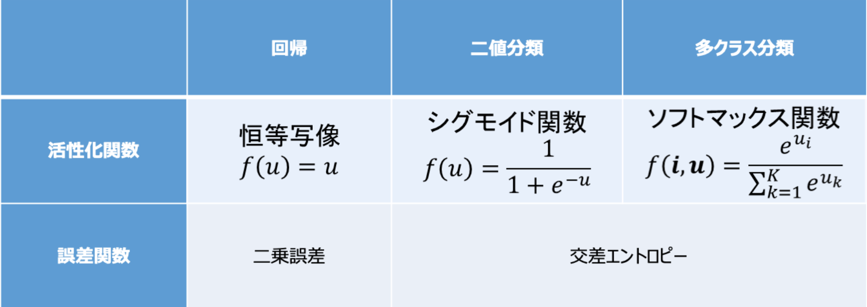
出力層の活性化関数

中間層と出力層の違い

• 中間層：しきい値の前後で信号の強弱を調整
• 出力層：信号の大きさをそのままに変更したり、０〜１を限定し、総和を１にしたりする

活性化関数＋誤差関数

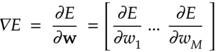
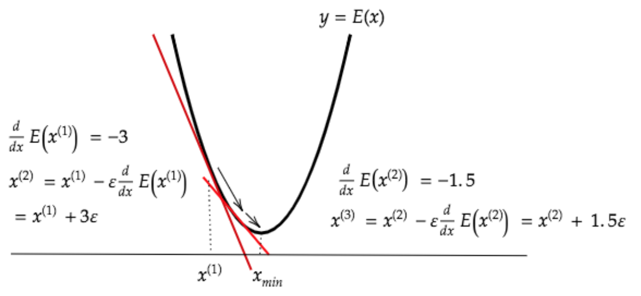
勾配降下法

深層学習の目的

学習を通して、誤差を最小にするネットワックを作る
いわば、誤差関数E(W)を最小化するパラメータWを探すこと

勾配降下法

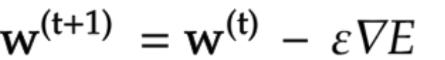
{\epsilon}学習率

学習率が大きすぎる

最小値にいつまでも、たどり着かず、発散してしまう

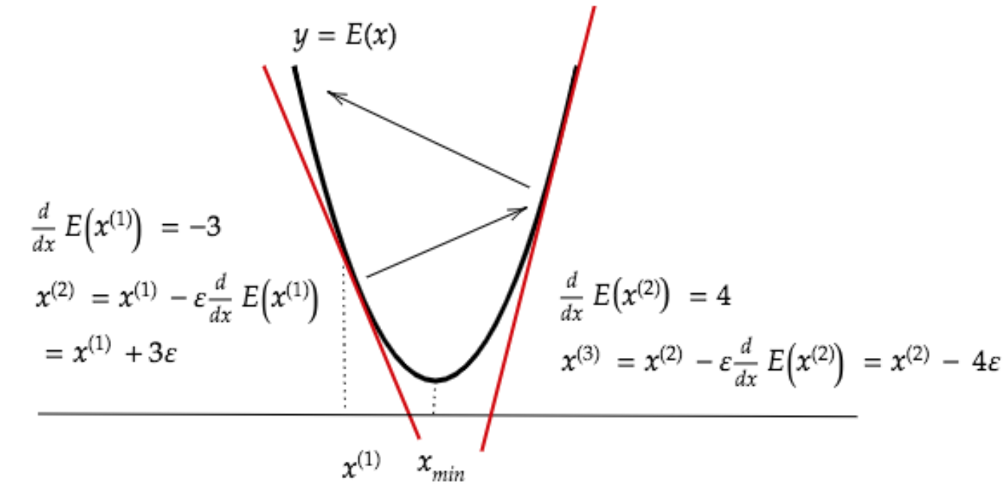
学習率が小さすぎる

学習する時間がかかる

学習率の決定、収束性向上のためのアルゴリズム

• Momentum
• AdaGrad
• AdaDelta
• Adam

確率的勾配降下法

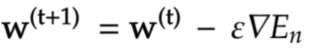
データ全体の誤差の代わり、ランダムに抽出したデータの誤差で計算する
以下のメリットがある

• 計算コストを軽減
• オンライ学習できる
• 局所的な最小値に収束するリスクを軽減
  ※オンライ学習：データ全体代わりに、随時、個別のデータを学習する

ミニバッチ勾配降下法

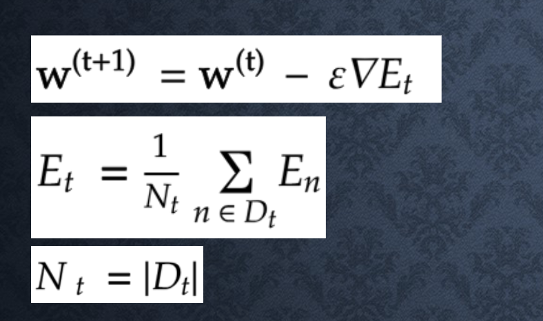
ランダムに分割したデータの集合（ミニバッチ）Dtに属するサンプルの平均誤差で計算する
並列計算を活用できるため、計算資源（CPU,GPU）を有効利用できる

数値微分

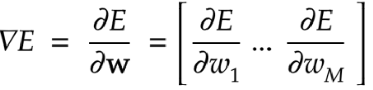
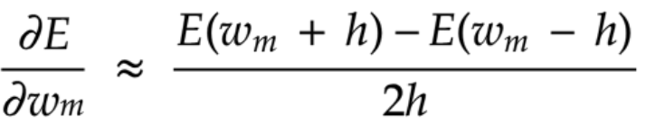
微小な数値を生成し擬似的に微分を計算する手法
どんな複雑な関数でも計算できる、
反面、各パラメータをそれぞれE(w+h)とE(w-h)を計算しないといけないため、
計算コストが高いすぎる
しかし、誤差逆伝播の結果を検証するのによく使われている

def numerical_gradient(f, x):
    h = 1e-4
    grad = np.zeros_like(x)

    for idx in range(x.size):
        tmp_val = x[idx]
        # f(x + h)の計算
        x[idx] = tmp_val + h
        fxh1 = f(x)

        # f(x - h)の計算
        x[idx] = tmp_val - h
        fxh2 = f(x)

        grad[idx] = (fxh1 - fxh2) / (2 * h)
        # 値を元に戻す
        x[idx] = tmp_val

    return grad

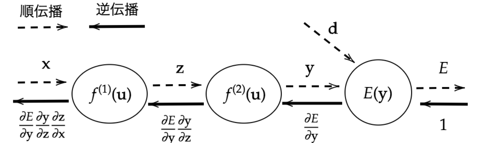
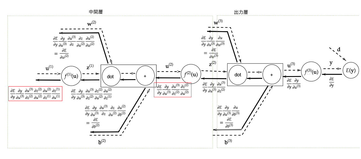
誤差逆伝播法

を計算するため、
算出された誤差を、出力層側から順に微分し、前の層へ、前の層へ伝播する
最小限の計算で各パラメータでの微分値を解析的に計算する手法

実装

初期設定

def init_network():
    # print("##### ネットワークの初期化 #####")
    network = {}
    nodesNum = 10
    network['W1'] = np.random.randn(2, nodesNum)
    network['W2'] = np.random.randn(nodesNum)
    network['b1'] = np.random.randn(nodesNum)
    network['b2'] = np.random.randn()

    return network

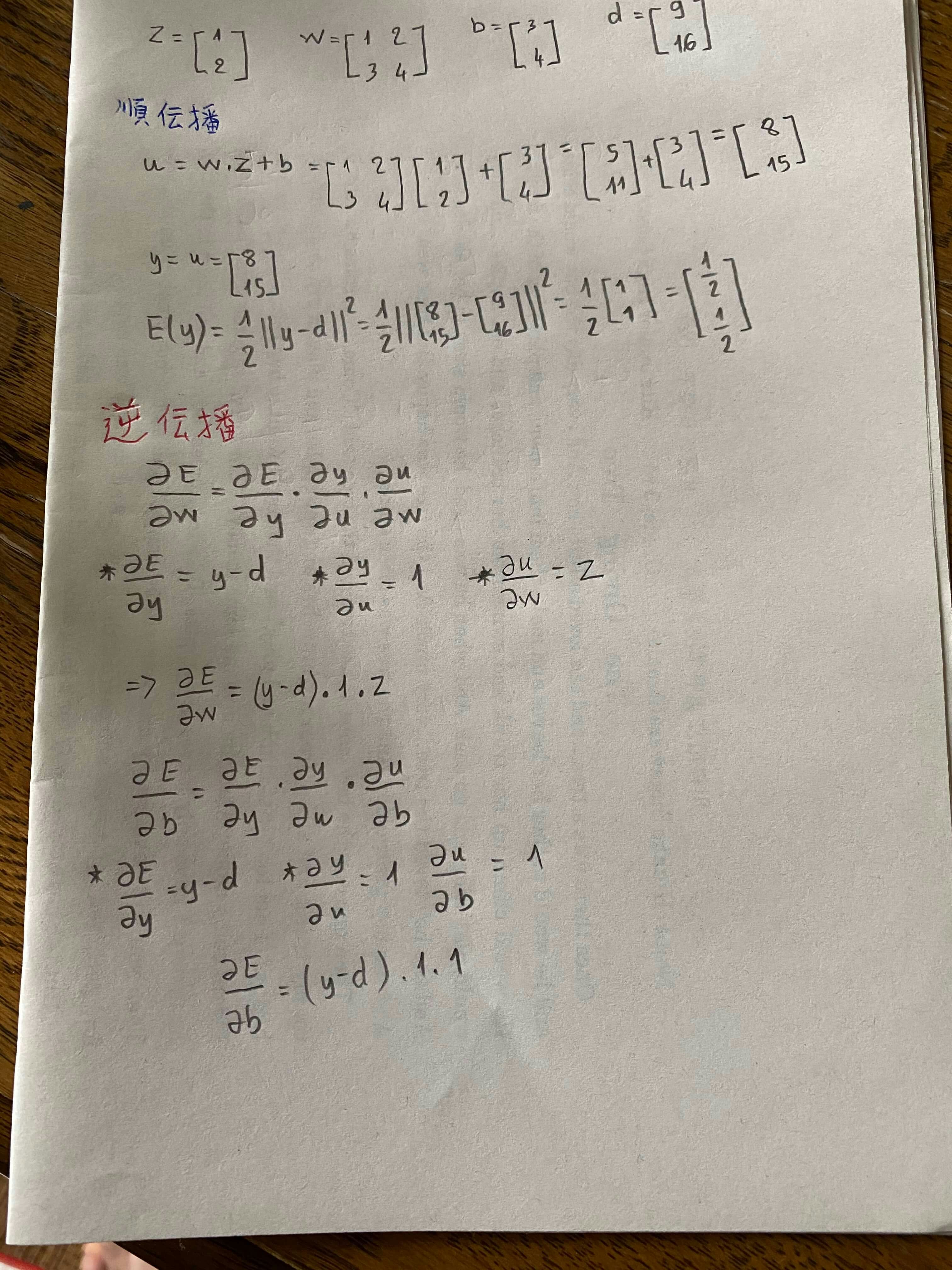
順伝播

def forward(network, x):
    # print("##### 順伝播開始 #####")
    
    W1, W2 = network['W1'], network['W2']
    b1, b2 = network['b1'], network['b2']
    u1 = np.dot(x, W1) + b1
    z1 = functions.relu(u1)
    
    u2 = np.dot(z1, W2) + b2
    y = u2
    
    return z1, y

逆伝播

# print("\n##### 誤差逆伝播開始 #####")    

    grad = {}
    
    W1, W2 = network['W1'], network['W2']
    b1, b2 = network['b1'], network['b2']

    # 出力層でのデルタ
    delta2 = functions.d_mean_squared_error(d, y)
    # b2の勾配
    grad['b2'] = np.sum(delta2, axis=0)

    # W2の勾配
    grad['W2'] = np.dot(z1.T, delta2)
    # 中間層でのデルタ
    delta1 = np.dot(delta2, W2.T) * functions.d_relu(z1)

    delta1 = delta1[np.newaxis, :]
    # b1の勾配
    grad['b1'] = np.sum(delta1, axis=0)
    x = x[np.newaxis, :]
    # W1の勾配
    grad['W1'] = np.dot(x.T, delta1)

    return grad

b1、b2の計算について

because the network is designed to process examples in (mini-)batches, and you therefore have gradients calculated for more than one example at a time. The sum is squashing the results down to a single update. This would be easier to confirm if you also showed update code for weights.

学習

def f(x):
    y = 3 * x[0] + 2 * x[1]
    return y
# サンプルデータを作成
data_sets_size = 100000
data_sets = [0 for i in range(data_sets_size)]

for i in range(data_sets_size):
    data_sets[i] = {}
    # ランダムな値を設定
    data_sets[i]['x'] = np.random.rand(2)
    
    ## 試してみよう_入力値の設定
    # data_sets[i]['x'] = np.random.rand(2) * 10 -5 # -5〜5のランダム数値
    
    # 目標出力を設定
    data_sets[i]['d'] = f(data_sets[i]['x'])
    
losses = []
# 学習率
learning_rate = 0.07

# 抽出数
epoch = 1000

# パラメータの初期化
network = init_network()
# データのランダム抽出
random_datasets = np.random.choice(data_sets, epoch)

# 勾配降下の繰り返し
for dataset in random_datasets:
    x, d = dataset['x'], dataset['d']
    z1, y = forward(network, x)
    grad = backward(x, d, z1, y)
    # パラメータに勾配適用
    for key in ('W1', 'W2', 'b1', 'b2'):
        network[key]  -= learning_rate * grad[key]

    # 誤差
    loss = functions.mean_squared_error(d, y)
    losses.append(loss)

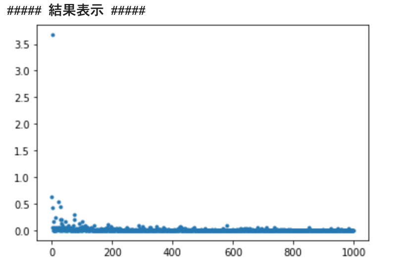
print("##### 結果表示 #####")    
lists = range(epoch)


plt.plot(lists, losses, '.')
# グラフの表示
plt.show()

#Day2

勾配消失問題

層が重ねれば重ねるほど、勾配降下法を用いると、
下位層のパラメータを更新するための勾配が小さくなりすぎ、
やがて、下位層のパラメータが更新できなくる問題

シグモイド関数の問題

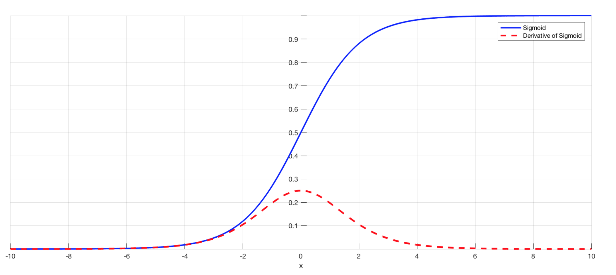
シグモイド関数を微分した最大値がたった0.25

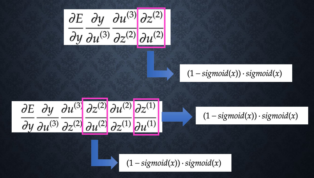
上記の式で勾配を計算すると何回も0.25を掛けたら、段々小さくなり、勾配消失が発生してしまう

勾配消失を解決する方法

活性化関数の選択

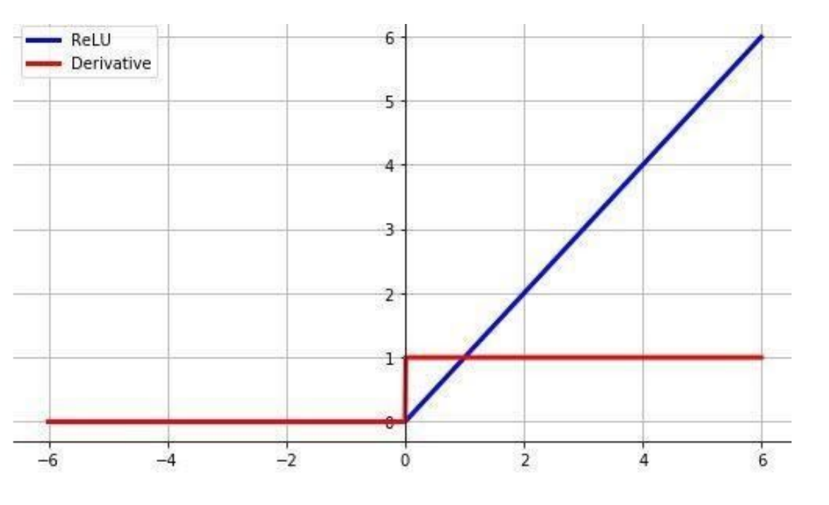
ReLU活性化関数の最大値が1で、最小値が0により、
勾配消失問題を抑止でき、スパース化に貢献できる

重みの初期値設定

y = w1x1 + w2x2 + ... + wNxN + b
重みw1,w2,...は普段、正規分布で初期化されているが、
yに対する活性関数の微分を大きすぎない（勾配爆発しない）、小さすぎない（勾配消失しない）ように、yの分散を重みの分散と近くように保つ手法。

Xavier

\frac{1}{\sqrt{n}}

network['W1'] = np.random.randn(input_layer_size, hidden_layer_1_size) / (np.sqrt(input_layer_size))

######利用する活性化関数

• ReLU
• Sigmoid
• Tanch(双曲線正接)

He

\frac{2}{\sqrt{n}}

network['W1'] = np.random.randn(input_layer_size, hidden_layer_1_size) / (np.sqrt(input_layer_size)) * np.sqrt(2)

######利用する活性化関数

• ReLU

考察

重みの初期値が0にすると、勾配消失が発生
1にすると、勾配爆発が発生
どの場合でも、うまく学習できない

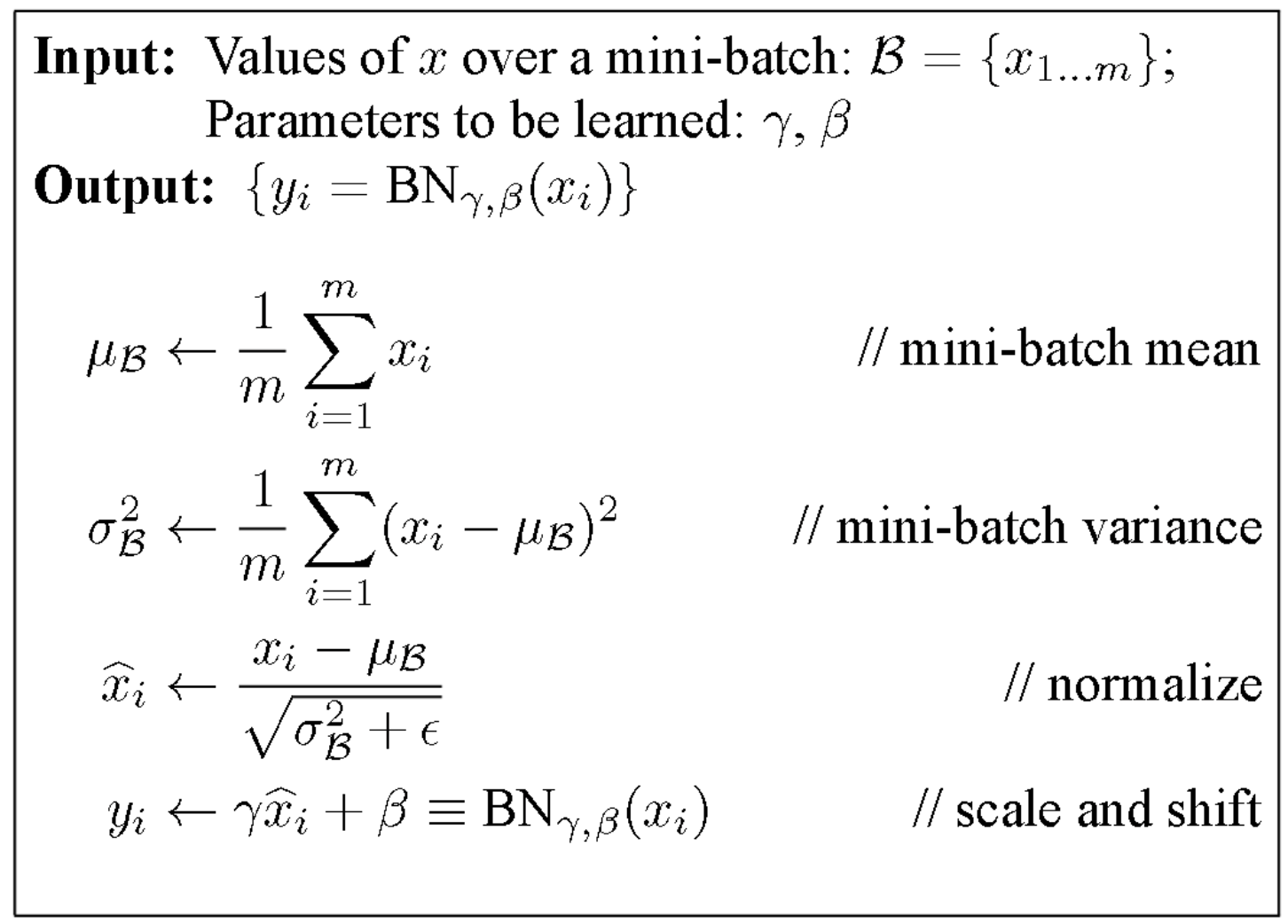
バッチの正規化

正規分布のように、入力値の偏りを調整する手法

数式

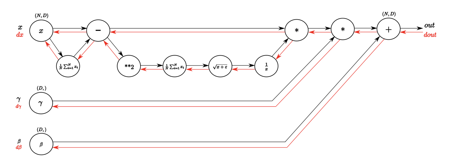
コード

Forward

def batchnorm_forward(x, gamma, beta, eps):

  N, D = x.shape

  #step1: calculate mean
  mu = 1./N * np.sum(x, axis = 0)

  #step2: subtract mean vector of every trainings example
  xmu = x - mu

  #step3: following the lower branch - calculation denominator
  sq = xmu ** 2

  #step4: calculate variance
  var = 1./N * np.sum(sq, axis = 0)

  #step5: add eps for numerical stability, then sqrt
  sqrtvar = np.sqrt(var + eps)

  #step6: invert sqrtwar
  ivar = 1./sqrtvar

  #step7: execute normalization
  xhat = xmu * ivar

  #step8: Nor the two transformation steps
  gammax = gamma * xhat

  #step9
  out = gammax + beta

  #store intermediate
  cache = (xhat,gamma,xmu,ivar,sqrtvar,var,eps)

  return out, cache

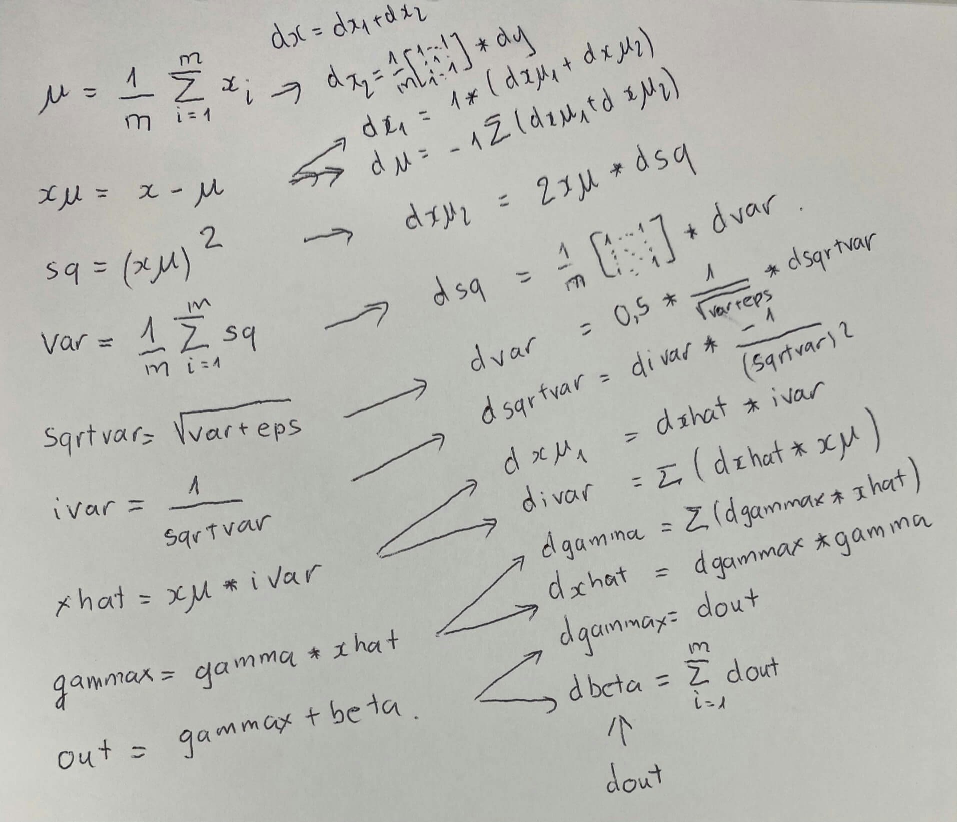
Backward

def batchnorm_backward(dout, cache):

  #unfold the variables stored in cache
  xhat,gamma,xmu,ivar,sqrtvar,var,eps = cache

  #get the dimensions of the input/output
  N,D = dout.shape

  #step9
  dbeta = np.sum(dout, axis=0)
  dgammax = dout #not necessary, but more understandable

  #step8
  dgamma = np.sum(dgammax*xhat, axis=0)
  dxhat = dgammax * gamma

  #step7
  divar = np.sum(dxhat*xmu, axis=0)
  dxmu1 = dxhat * ivar

  #step6
  dsqrtvar = -1. /(sqrtvar**2) * divar

  #step5
  dvar = 0.5 * 1. /np.sqrt(var+eps) * dsqrtvar

  #step4
  dsq = 1. /N * np.ones((N,D)) * dvar

  #step3
  dxmu2 = 2 * xmu * dsq

  #step2
  dx1 = (dxmu1 + dxmu2)
  dmu = -1 * np.sum(dxmu1+dxmu2, axis=0)

  #step1
  dx2 = 1. /N * np.ones((N,D)) * dmu

  #step0
  dx = dx1 + dx2

  return dx, dgamma, dbeta

効果

• 多少ノイズがInputに追加されたため、過学習の抑止を期待できる。
• 学習率を大きく設定しても、Inputが正規化されたため、勾配消失・爆発を抑えられる。

学習率最適化手法

勾配降下法

w^{(t+1)} = w^{(t)} - \epsilon\Delta E

モメンタム

V_{t} = \mu V_{t-1}  - \epsilon\Delta E\\
w^{(t+1)} = w^{(t)} + V_{t}\\
\mu :慣性

class Momentum:
    def __init__(self, learning_rate=0.01, momentum=0.9):
        self.learning_rate = learning_rate
        self.momentum = momentum
        self.v = None
        
    def update(self, params, grad):
        if self.v is None:
            self.v = {}
            for key, val in params.items():                                
                self.v[key] = np.zeros_like(val)
                
        for key in params.keys():
            self.v[key] = self.momentum * self.v[key] - self.learning_rate * grad[key] 
            params[key] += self.v[key]

特徴

• 局所的最適解にならず、大局的最適解となる
• 最適値に行くまでの時間が早い

AdaGrad

h_{t} = h_{t-1}  + (\Delta E)^2\\
w^{(t+1)} = w^{(t)}  - \epsilon \frac{1}{\sqrt{h_{t}}} \Delta E\\

class AdaGrad:
    def __init__(self, learning_rate=0.01):
        self.learning_rate = learning_rate
        self.h = None
        
    def update(self, params, grad):
        if self.h is None:
            self.h = {}
            for key, val in params.items():
                self.h[key] = np.zeros_like(val)
            
        for key in params.keys():
            self.h[key] += grad[key] * grad[key]
            params[key] -= self.learning_rate * grad[key] / (np.sqrt(self.h[key]) + 1e-7)

特徴

• 勾配の穏やかな斜面に対して、最適値に近いづける
• 学習率が徐々に小さくなるため、鞍点問題が起こることもある

RMSProp

h_{t} = \alpha h_{t-1}  + (1 -\alpha)(\Delta E)^2\\
w^{(t+1)} = w^{(t)}  - \epsilon \frac{1}{\sqrt{h_{t}} + \theta} \Delta E\\

class RMSprop:
    def __init__(self, learning_rate=0.01, decay_rate = 0.99):
        self.learning_rate = learning_rate
        self.decay_rate = decay_rate
        self.h = None
        
    def update(self, params, grad):
        if self.h is None:
            self.h = {}
            for key, val in params.items():
                self.h[key] = np.zeros_like(val)
            
        for key in params.keys():
            self.h[key] *= self.decay_rate
            self.h[key] += (1 - self.decay_rate) * grad[key] * grad[key]
            params[key] -= self.learning_rate * grad[key] / (np.sqrt(self.h[key]) + 1e-7)

特徴

• 局所的最適解にならず、大局的最適解となる
• AdaGradの進化系
• AdaGradに比べたら、ハイパーパラメーターの調整が少ない

Adam

モメンタムの、過去の勾配の指数関数的減衰平均と
RMSPropの、過去の勾配の２乗の指数関数的減衰平均を
孕んだ最適化アルゴリズム

m_{t} = \beta_{1} m_{t-1}  + (1 -\beta_{1})\Delta E\\
v_{t} = \beta_{2} v_{t-1}  + (1 -\beta_{2})(\Delta E)^2\\
w^{(t+1)} = w^{(t)}  - \epsilon \frac{m_{t}}{\sqrt{v_{t}} + \theta} \\

class Adam:
    def __init__(self, learning_rate=0.001, beta1=0.9, beta2=0.999):
        self.learning_rate = learning_rate
        self.beta1 = beta1
        self.beta2 = beta2
        self.iter = 0
        self.m = None
        self.v = None
        
    def update(self, params, grad):
        if self.m is None:
            self.m, self.v = {}, {}
            for key, val in params.items():
                self.m[key] = np.zeros_like(val)
                self.v[key] = np.zeros_like(val)
        
        self.iter += 1
        lr_t  = self.learning_rate * np.sqrt(1.0 - self.beta2 ** self.iter) / (1.0 - self.beta1 ** self.iter)         
        
        for key in params.keys():
            self.m[key] += (1 - self.beta1) * (grad[key] - self.m[key])
            self.v[key] += (1 - self.beta2) * (grad[key] ** 2 - self.v[key])
            
            params[key] -= lr_t * self.m[key] / (np.sqrt(self.v[key]) + 1e-7)

過学習

原因

• 学習データに対して、パラメーター数が圧倒的に多い
• パラメーターの値が適切ではない
• ノード（層）が多い

正則化

過学習を抑止するため、ネットワークの（パラメーター、層など）を制約する

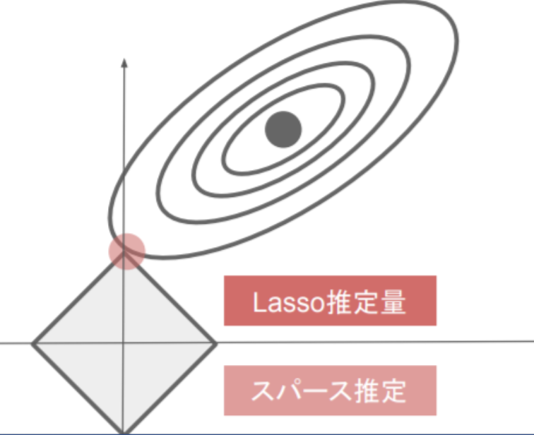
L1正則化-Lasso

\|W\|_1 = (| w_1| + | w_2| +...+ | w_n|)\\
E_n(W) + \lambda \|W\|_1\\

λ:weight_decay_lambda

ソース

# 正則化強度設定 ======================================
weight_decay_lambda = 0.005
# =================================================

for i in range(iters_num):
    batch_mask = np.random.choice(train_size, batch_size)
    x_batch = x_train[batch_mask]
    d_batch = d_train[batch_mask]

    grad = network.gradient(x_batch, d_batch)
    weight_decay = 0
    
    for idx in range(1, hidden_layer_num+1):
        grad['W' + str(idx)] = network.layers['Affine' + str(idx)].dW + weight_decay_lambda * np.sign(network.params['W' + str(idx)])
        grad['b' + str(idx)] = network.layers['Affine' + str(idx)].db
        network.params['W' + str(idx)] -= learning_rate * grad['W' + str(idx)]
        network.params['b' + str(idx)] -= learning_rate * grad['b' + str(idx)]        
        weight_decay += weight_decay_lambda * np.sum(np.abs(network.params['W' + str(idx)]))

    loss = network.loss(x_batch, d_batch) + weight_decay
    train_loss_list.append(loss)  

解説

正則化付き勾配

grad[W] = grad[w] + λ *np.sign(W)

grad['W' + str(idx)] = network.layers['Affine' + str(idx)].dW + weight_decay_lambda * np.sign(network.params['W' + str(idx)])

損失計算

weight_decay = 0    
for idx in range(1, hidden_layer_num+1):
    ...       
    weight_decay += weight_decay_lambda * np.sum(np.abs(network.params['W' + str(idx)]))
loss = network.loss(x_batch, d_batch) + weight_decay

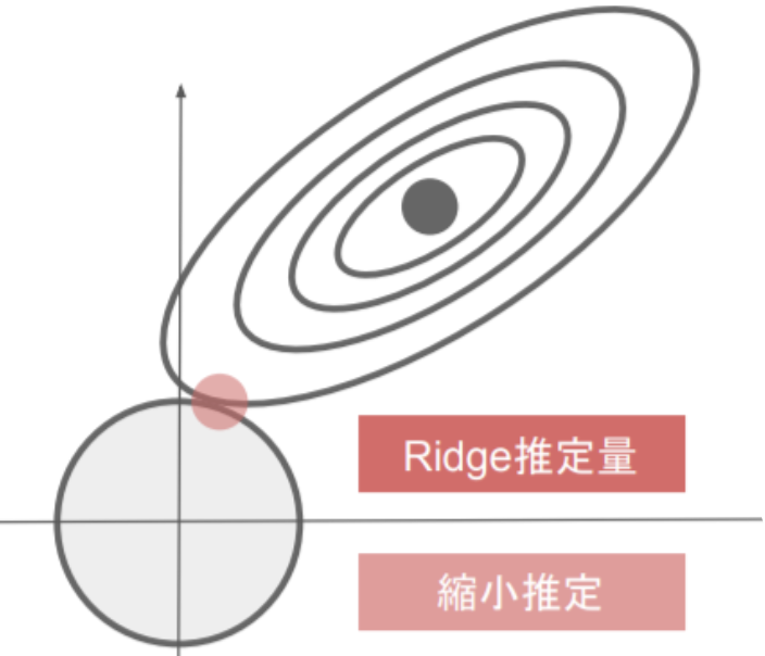
L2正則化-Ridge

\|W\|_2 = \sqrt{(| w_1|^2 + | w_2|^2 +...+ | w_n|^2)}\\
E_n(W) + \frac{1}{2} \lambda \|W\|_2\\

λ:weight_decay_lambda

ソース

# 正則化強度設定 ======================================
weight_decay_lambda = 0.1
# =================================================

for i in range(iters_num):
    batch_mask = np.random.choice(train_size, batch_size)
    x_batch = x_train[batch_mask]
    d_batch = d_train[batch_mask]

    grad = network.gradient(x_batch, d_batch)
    weight_decay = 0
    
    for idx in range(1, hidden_layer_num+1):
        grad['W' + str(idx)] = network.layers['Affine' + str(idx)].dW + weight_decay_lambda * network.params['W' + str(idx)]
        grad['b' + str(idx)] = network.layers['Affine' + str(idx)].db
        network.params['W' + str(idx)] -= learning_rate * grad['W' + str(idx)]
        network.params['b' + str(idx)] -= learning_rate * grad['b' + str(idx)]        
        weight_decay += 0.5 * weight_decay_lambda * np.sqrt(np.sum(network.params['W' + str(idx)] ** 2))

    loss = network.loss(x_batch, d_batch) + weight_decay
    train_loss_list.append(loss) 

解説

正則化付き勾配

grad[W] = grad[w] + λ *W

grad['W' + str(idx)] = network.layers['Affine' + str(idx)].dW + weight_decay_lambda * network.params['W' + str(idx)]

損失計算

weight_decay = 0
for idx in range(1, hidden_layer_num+1):
   ...       
   weight_decay += 0.5 * weight_decay_lambda * np.sqrt(np.sum(network.params['W' + str(idx)] ** 2))
loss = network.loss(x_batch, d_batch) + weight_decay

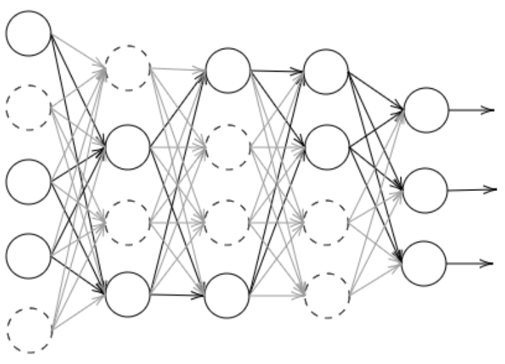
ドロップアウト

ランダムにノードを削除し、学習する

ソース

class Dropout:
    def __init__(self, dropout_ratio=0.5):
        self.dropout_ratio = dropout_ratio
        self.mask = None

    def forward(self, x, train_flg=True):
        if train_flg:
            self.mask = np.random.rand(*x.shape) > self.dropout_ratio
            return x * self.mask
        else:
            return x * (1.0 - self.dropout_ratio)

    def backward(self, dout):
        return dout * self.mask

学習結果

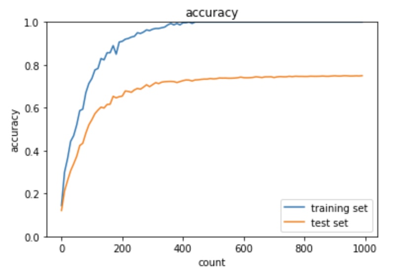
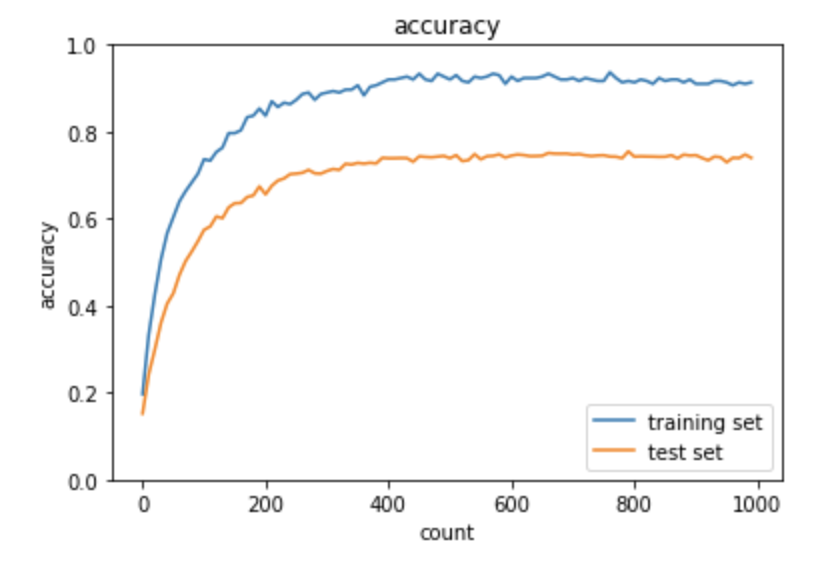
過学習

学習データに対する正解率が1.0に達しているが、
テストデータに対する正解率が0.65前後に止まっている。

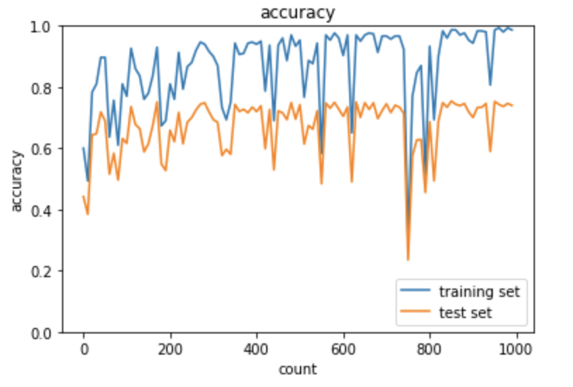
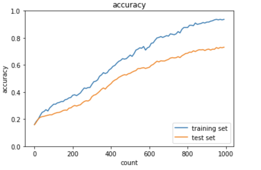
L1正則化

スパース化の影響により、正解率の変動幅が激しくなり、
過学習が多少改善できている

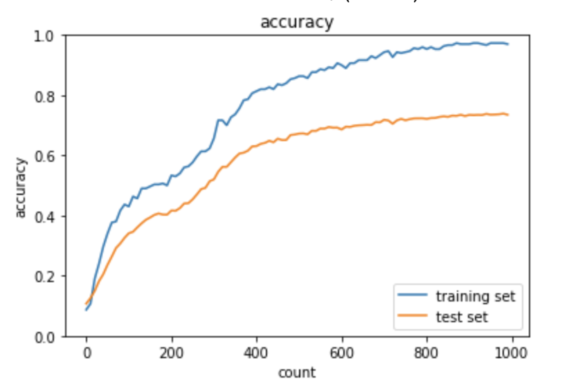
L2正則化

学習データに対する正解率が1.0に達していないが、
テストデータに対する正解率も0.65前後に止まっている。

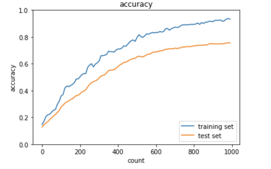
ドロップアウト

滑らかに学習できている

ドロップアウト+L1正則化

ドロップアウト+L2正則化

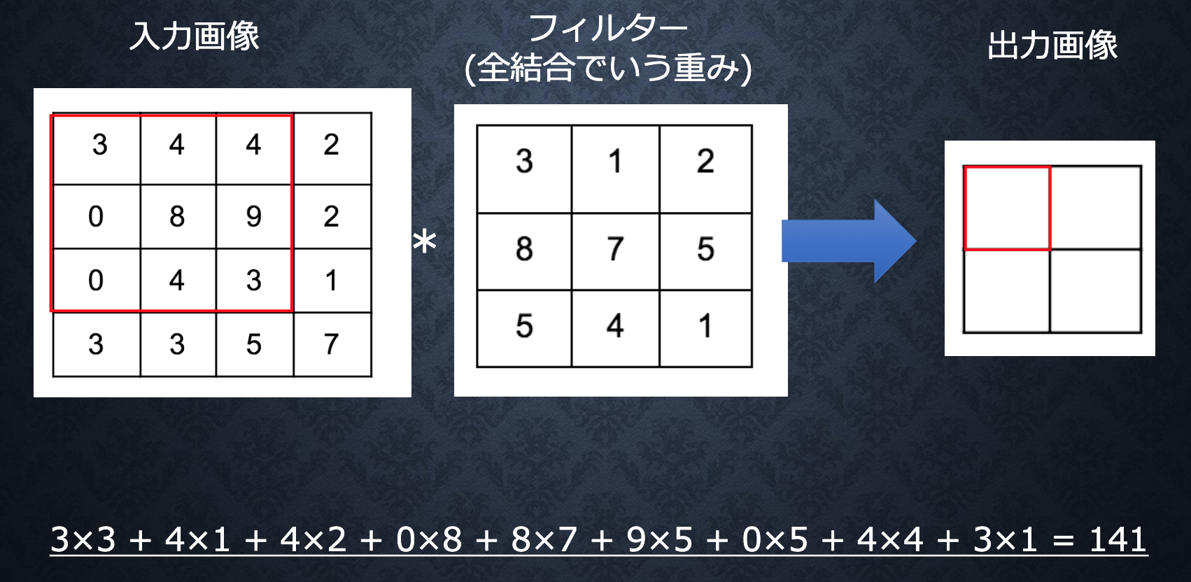
畳み込みニューラルネットワークの概念

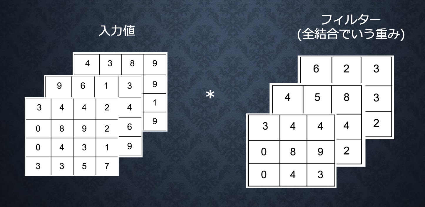
畳み込み層

写真のデータだと、縦・横・チャネルが存在しているため、
１次元の配列に変化すると、左、上、右、下のピクセルの関係がなくなる。
畳み込み層を利用すると、そういう関係を保ちつつ、学習できる。

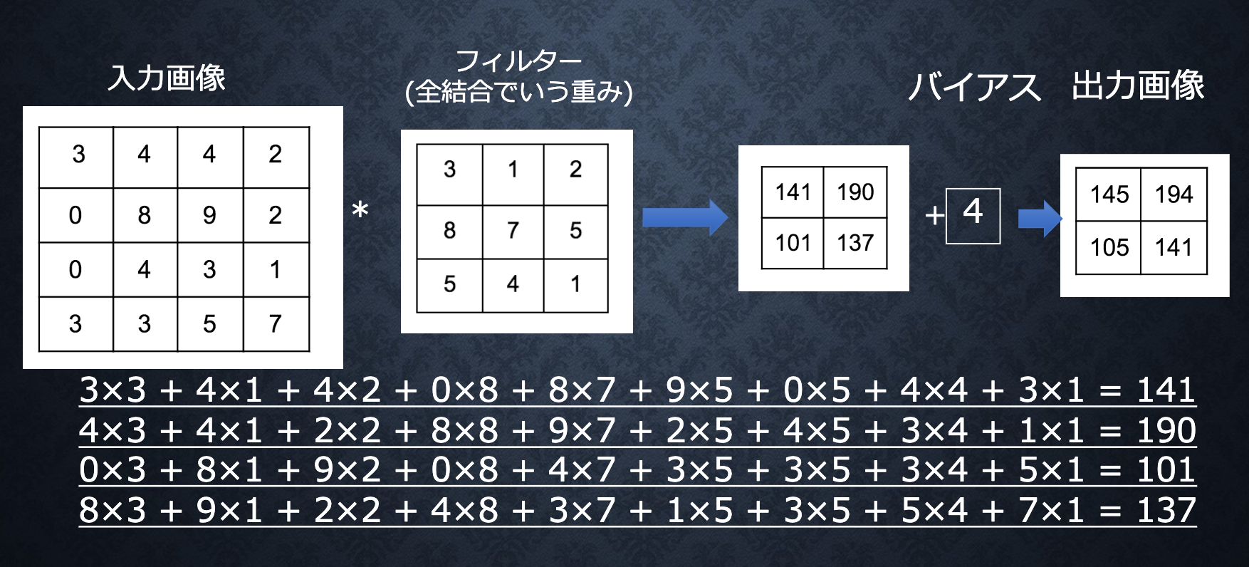
演算概念

バイアス

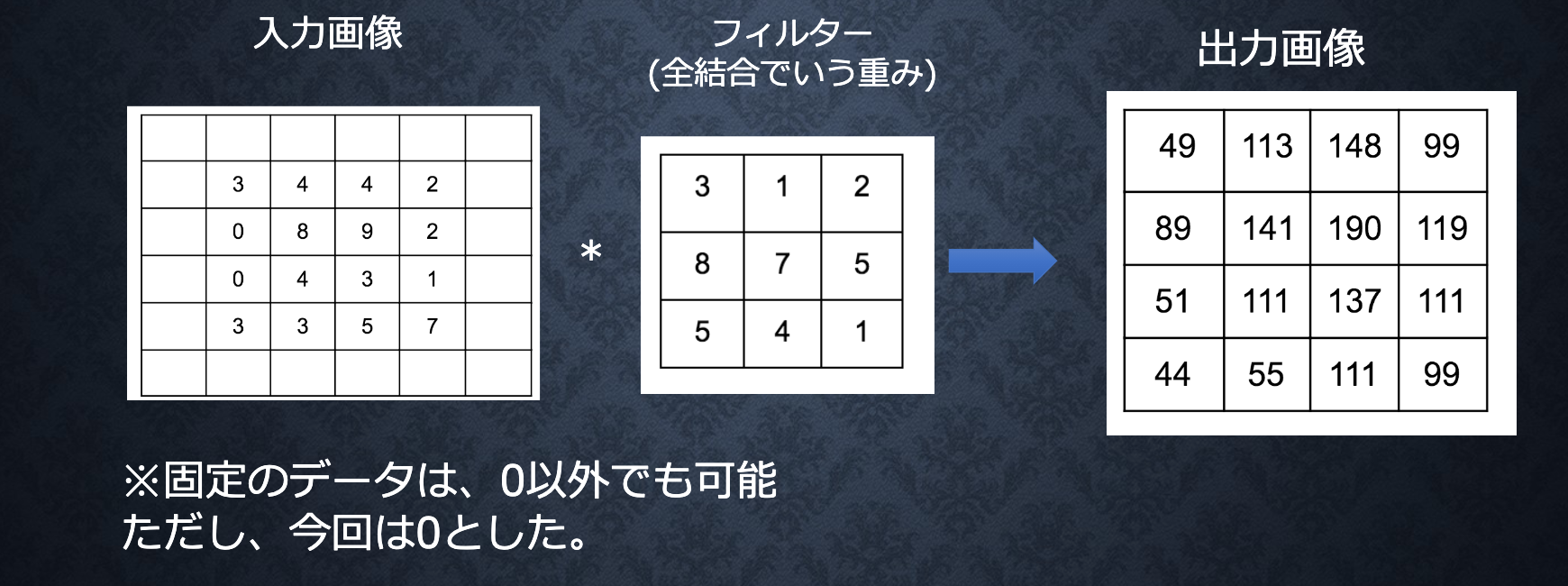
パディング

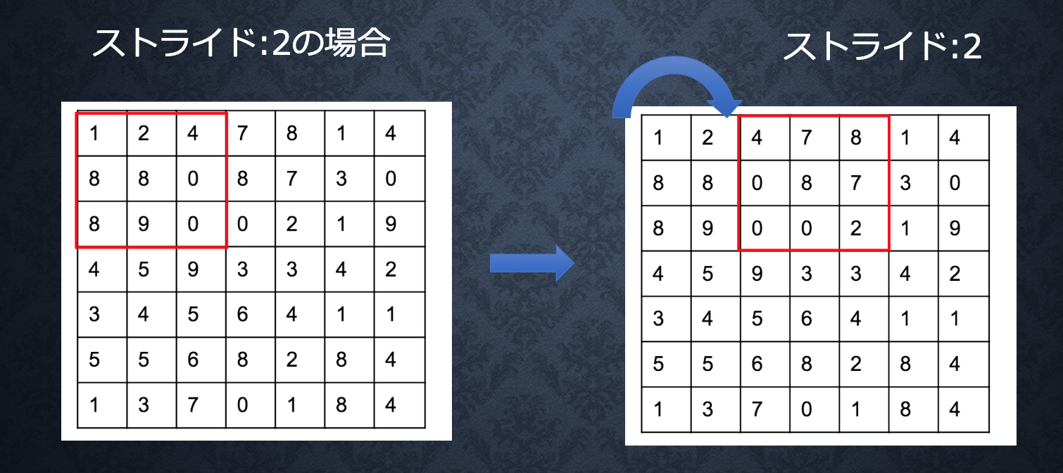
ストライド

チャンネル

出力サイズの計算

出力値のheight, width

#入力
input_h
input_w

#フィルタ
filter_h
filter_w

#パディング
padding

#ストライド
stride

#出力
output_h
output_w

#算出
output_h = 1 + int((input_h + 2 * padding - filter_h) / stride)
output_w = 1 + int((input_w + 2 * padding - filter_w) / stride)

ソース

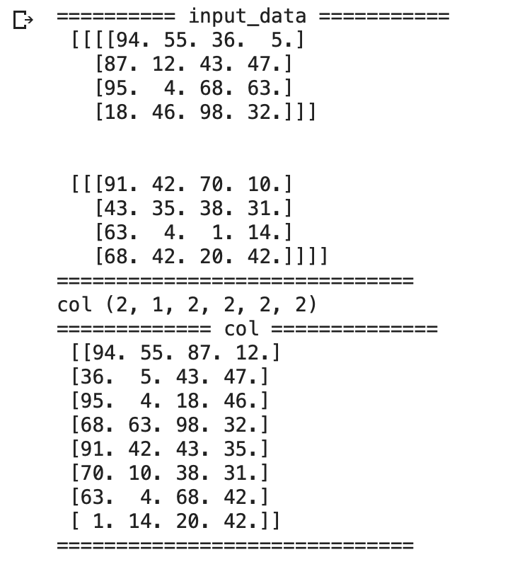
im2col

# 画像データを２次元配列に変換
'''
input_data: 入力値
filter_h: フィルターの高さ
filter_w: フィルターの横幅
stride: ストライド
pad: パディング
'''
def im2col(input_data, filter_h, filter_w, stride=1, pad=0):
    # N: number, C: channel, H: height, W: width
    N, C, H, W = input_data.shape
    out_h = (H + 2 * pad - filter_h)//stride + 1
    out_w = (W + 2 * pad - filter_w)//stride + 1

    img = np.pad(input_data, [(0,0), (0,0), (pad, pad), (pad, pad)], 'constant')
    col = np.zeros((N, C, filter_h, filter_w, out_h, out_w))
    for y in range(filter_h):
        y_start = y 
        y_max = y_start + stride * out_h
        for x in range(filter_w):
            x_start = x 
            x_max = x_start + stride * out_w
            col[:, :, y, x, :, :] = img[:, :, y_start:y_max:stride, x_start:x_max:stride]
    col = col.transpose(0, 4, 5, 1, 2, 3) # (N, C, filter_h, filter_w, out_h, out_w) -> (N, filter_w, out_h, out_w, C, filter_h)   
    col = col.reshape(N * out_h * out_w, -1)
    return col

確認

input_data = np.random.rand(2, 1, 4, 4)*100//1 # number, channel, height, widthを表す
print('========== input_data ===========\n', input_data)
print('==============================')
filter_h = 2
filter_w = 2
stride = 2
pad = 0
col = im2col(input_data, filter_h=filter_h, filter_w=filter_w, stride=stride, pad=pad)
print('============= col ==============\n', col)
print('==============================')

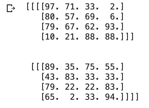
col2im

# ２次元配列を画像データに変換
def col2im(col, input_shape, filter_h, filter_w, stride=1, pad=0):
    # N: number, C: channel, H: height, W: width
    N, C, H, W = input_shape
    # 切り捨て除算    
    out_h = (H + 2 * pad - filter_h)//stride + 1
    out_w = (W + 2 * pad - filter_w)//stride + 1
    col = col.reshape(N, out_h, out_w, C, filter_h, filter_w).transpose(0, 3, 4, 5, 1, 2) # (N, filter_h, filter_w, out_h, out_w, C)
    img = np.zeros((N, C, H + 2 * pad + stride - 1, W + 2 * pad + stride - 1))
    for y in range(filter_h):
        y_max = y + stride * out_h
        for x in range(filter_w):
            x_max = x + stride * out_w
            img[:, :, y:y_max:stride, x:x_max:stride] = col[:, :, y, x, :, :]

    return img[:, :, pad:H + pad, pad:W + pad]

確認

img = col2im(col, input_shape=(2, 1, 4, 4),filter_h=filter_h, filter_w=filter_w, stride=stride, pad=pad)
print(img)

Convolution

class Convolution:
    # W: フィルター, b: バイアス
    def __init__(self, W, b, stride=1, pad=0):
        self.W = W
        self.b = b
        self.stride = stride
        self.pad = pad
        
        # 中間データ（backward時に使用）
        self.x = None   
        self.col = None
        self.col_W = None
        
        # フィルター・バイアスパラメータの勾配
        self.dW = None
        self.db = None

    def forward(self, x):
        # FN: filter_number, C: channel, FH: filter_height, FW: filter_width
        FN, C, FH, FW = self.W.shape
        N, C, H, W = x.shape
        # 出力値のheight, width
        out_h = 1 + int((H + 2 * self.pad - FH) / self.stride)
        out_w = 1 + int((W + 2 * self.pad - FW) / self.stride)
        
        # xを行列に変換
        col = im2col(x, FH, FW, self.stride, self.pad)
        # フィルターをxに合わせた行列に変換
        col_W = self.W.reshape(FN, -1).T
        print('col',col.shape)
        print('col_W',col_W.shape)
        out = np.dot(col, col_W) + self.b
        # 計算のために変えた形式を戻す
        out = out.reshape(N, out_h, out_w, -1).transpose(0, 3, 1, 2)
        print('out',out.shape)
        self.x = x
        self.col = col
        self.col_W = col_W

        return out

    def backward(self, dout):
        FN, C, FH, FW = self.W.shape
        dout = dout.transpose(0, 2, 3, 1).reshape(-1, FN)

        self.db = np.sum(dout, axis=0)
        self.dW = np.dot(self.col.T, dout)
        self.dW = self.dW.transpose(1, 0).reshape(FN, C, FH, FW)

        dcol = np.dot(dout, self.col_W.T)
        # dcolを画像データに変換
        dx = col2im(dcol, self.x.shape, FH, FW, self.stride, self.pad)

        return dx

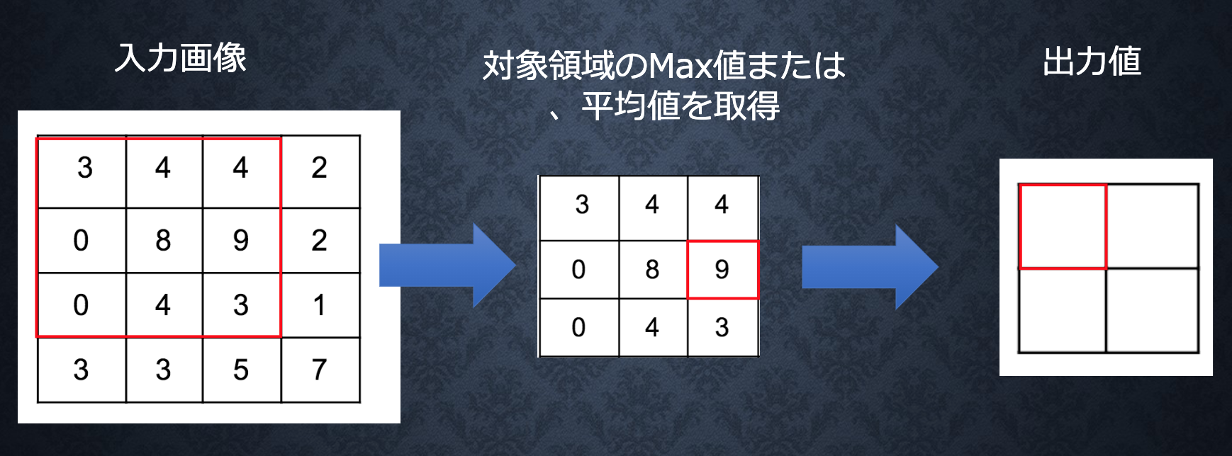
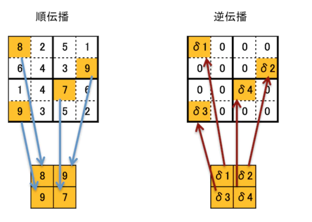
プーリング層

ソース

class Pooling:
    def __init__(self, pool_h, pool_w, stride=1, pad=0):
        self.pool_h = pool_h
        self.pool_w = pool_w
        self.stride = stride
        self.pad = pad
        
        self.x = None
        self.arg_max = None

    def forward(self, x):
        N, C, H, W = x.shape
        out_h = int(1 + (H - self.pool_h) / self.stride)
        out_w = int(1 + (W - self.pool_w) / self.stride)
        
        # xを行列に変換
        col = im2col(x, self.pool_h, self.pool_w, self.stride, self.pad)
        # プーリングのサイズに合わせてリサイズ
        col = col.reshape(-1, self.pool_h*self.pool_w)
        
        # 行ごとに最大値を求める
        arg_max = np.argmax(col, axis=1)
        out = np.max(col, axis=1)
        # 整形
        out = out.reshape(N, out_h, out_w, C).transpose(0, 3, 1, 2)

        self.x = x
        self.arg_max = arg_max

        return out

    def backward(self, dout):
        dout = dout.transpose(0, 2, 3, 1)
        
        pool_size = self.pool_h * self.pool_w
        dmax = np.zeros((dout.size, pool_size))
        dmax[np.arange(self.arg_max.size), self.arg_max.flatten()] = dout.flatten()
        dmax = dmax.reshape(dout.shape + (pool_size,)) 
        
        dcol = dmax.reshape(dmax.shape[0] * dmax.shape[1] * dmax.shape[2], -1)
        dx = col2im(dcol, self.x.shape, self.pool_h, self.pool_w, self.stride, self.pad)
        
        return dx

最新CNN

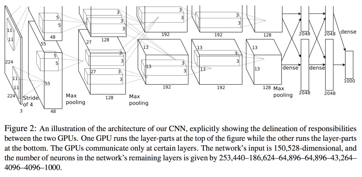
AlexNet

####　概要
2012年、ヒントン 教授チームに発表される物体認識のモデル
初の深層学習概念を取り組むモデル
####　構造
input:224×224×3の写真
output:1000個の要素を持つ一次元の配列

畳み込み層：5
プーリング層：3
全結合層：３

####　ソース・Keras

#Alex net
model = Sequential()

# Layer 1
model.add(Conv2D(48, kernel_size=(11, 11), strides=(4,4), input_shape=(224, 224, 3),activation='relu'))
model.add(MaxPooling2D(pool_size=(2, 2), strides=(2,2), padding='same'))
model.add(BatchNormalization())

# Layer 2
model.add(Conv2D(128, kernel_size=(5, 5), activation='relu'))
model.add(MaxPooling2D(pool_size=(2, 2), strides=(2,2), padding='same'))
model.add(BatchNormalization())

# Layer 3
model.add(Conv2D(192, kernel_size=(3, 3), activation='relu'))
model.add(BatchNormalization())

# Layer 4
model.add(Conv2D(192, kernel_size=(3, 3), activation='relu'))
model.add(BatchNormalization())

# Layer 5
model.add(Conv2D(128, kernel_size=(3, 3), activation='relu'))
model.add(MaxPooling2D(pool_size=(2, 2), strides=(2,2), padding='same'))
model.add(BatchNormalization())

model.add(Flatten())

# Layer 6
model.add(Dense(2048, activation='relu'))
model.add(BatchNormalization())
model.add(Dropout(0.01))

# Layer 7
model.add(Dense(2048, activation='relu'))
model.add(BatchNormalization())
model.add(Dropout(0.01))

# Layer 8
model.add(Dense(1000, activation="softmax"))

model.summary()
model.compile(optimizer=keras.optimizers.Adam(lr=0.001), 
                loss='categorical_crossentropy',
                metrics = ['accuracy'])