追記:入門①~③を実質まとめたような記事を書きました
[拡散モデル入門] ゼロから理解する拡散モデルの最新理論(図解付き)
入門①:DDPMの理論とMNISTの実装
入門②:SDE/ODEの基礎理論(Tensorflow実装付き)
入門③:EDMの解説とMNISTの実装
入門④:ここ
応用編:拡散モデルにGRPOを使ってファインチューニングしてみた
最後にU-Netの詳細と条件の埋め込み方について見ていきます。
参考
・https://huggingface.co/blog/annotated-diffusion
・https://github.com/eloialonso/diamond/
DDPMベースのU-Net
DDPMの実装ではU-Netに Wide ResNet block の使用、Attention層の追加、バッチ正規化からグループ正規化への変更がされています。
EDMでもU-Netの実装自体は変わりはないようです。
本記事では、細かい違いはありますが内部でEDMが使われているDIAMONDの実装(GitHub)をベースに見ていきます。
全体から各モジュールに掘り下げる形で見ていきます。
U-Net
U-Netは画像を入力として画像を出力するモデルとなります。
解像度を下げるDownsampleと解像度を上げるUpsample、それらを直接つなげるスキップ接続(Skip Connection)があるのが特徴です。

画像に情報を付与する場合は、条件付けとして Condition を入力します。
Conditionは全部の層に対して入力されます。
また、ブロックの順序ですがネットの実装を見てみると "Down/Up→ResBlock" と "ResBock→Down/Up" の両方の実装が見られました。
違いが分からなかったのでChatGPTに聞いたところ以下のようです。
| 順序 | 特徴 | メリット/デメリット | 例 |
|---|---|---|---|
| ResBlock → Downsample | 特徴を先に抽出してから縮小 | 計算コストが高いが、高解像度の情報を保持 | DDPM,画像生成 |
| Downsample → ResBlock | 縮小してから特徴抽出 | 計算コストが低いが、情報の損失が大きい | 分類モデル,小規模な特徴抽出 |
| 順序 | 特徴 | メリット | デメリット | 例 |
|---|---|---|---|---|
| ResBlock → Upsample | 特徴を先に抽出し、拡大する | 高解像度の情報を保持しやすい | アップサンプリング後の調整が少ない | DDPM,画像生成 |
| Upsample → ResBlock | 先に拡大し、特徴を再調整 | 高解像度の特徴を学習できる | 拡大時の情報損失が大きくなる可能性 | 超解像, 高解像度の画像処理 |
Condition
Condition は各画像の追加情報で、拡散モデルのタイムステップの情報も含まれます。
今回はMNISTのカテゴリ情報も追加してみました。
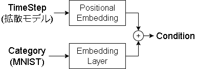
タイムステップはDIAMONDの実装ではフーリエ変換された特徴量を使っていましたが、この記事ではDDPMに倣ってサインコサインエンコーディングにしています。
MNISTのカテゴリ情報はTFのEmbbedingレイヤーでベクトル化しました。
Downsample/Upsample
DIAMONDの実装では、DownsampleはConv2Dのstrides=2でサイズを半分にし、Upsampleは最近傍補間で2倍にしていましたので、それに倣っています。
class Downsample(keras.layers.Layer):
    def build(self, input_shape):
        self.conv = kl.Conv2D(
            filters=input_shape[-1],
            kernel_size=3,
            strides=2,
            padding="same",
            kernel_initializer=keras.initializers.Orthogonal(),
        )

    def call(self, x, training=False):
        return self.conv(x, training=training)

class Upsample(keras.layers.Layer):
    def build(self, input_shape):
        self.conv = kl.Conv2D(
            filters=input_shape[-1],
            kernel_size=3,
            strides=1,
            padding="same",
        )

    def call(self, x, training=False):
        # 最近傍補間で2倍にリサイズ
        input_shape = tf.shape(x)
        x = tf.image.resize(x, size=(input_shape[1] * 2, input_shape[2] * 2), method="nearest")
        return self.conv(x, training=training)
ResBLocks & ResBlock(Residual Block)
ResBLocksですが、複数のResBlockから成ります。
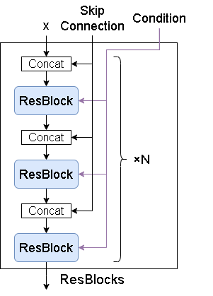
Skip Connection は Upsample にのみあり Downsample の出力に対応します。
次にResBlockです。

普通のResBlockと違う点は最後にAttentionレイヤー(SelfAttention)が入っている点です。
またConditionですが、DDPMではConv3x3層に直接足していましたが、DIAMONDでは AdaGN としてNorm層に追加しています。
Adaptive Group Normalization(AdaGN)
Normレイヤーですが、一般的には Group Normalization(GN)が使われます。
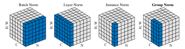
図はGroup Normalization (論文)より、他の正規化手法とGNの違いを表しており、Nがバッチ、Cがチャンネル、(H,W)が画像を表す軸となります。
簡単にまとめると以下です。
| Norm | バッチ軸 | チャンネル軸 | |
|---|---|---|---|
| Batch Norm | All | 1 | バッチに対して正規化 |
| Layer Norm | 1 | All | チャンネルに対して正規化 |
| Instance Norm | 1 | 1 | 画像チャンネル毎に正規化 |
| Group Norm | 1 | グループで分割 | チャンネル軸を分割し、それぞれのグループで正規化 |
DIAMONDの実装では GN ではなく、Adaptive Group Normalization(AdaGN)が使われていました。
これは GN に条件(例えばスタイル情報など)を適用できるように拡張した手法です。
GN は以下のように正規化されます。
$$
\hat{x}_i = \frac{x_i - \mu_g}{\sigma_g}
$$
$\mu_g$と$\sigma_g$がグループ$g$の平均と標準偏差を表します。
AdaGNではこれに条件 $s$ に対するスケール $\gamma$ とバイアス $\beta$ が追加されます。
$$
\hat{x}_i = \gamma(s)\cdot \frac{x_i - \mu_g}{\sigma_g} + \beta(s)
$$
主にスタイル変換(Style Transfer)や今回みたいな条件付画像生成で使われることが多いようです。
多分これが論文:Arbitrary Style Transfer in Real-time with Adaptive Instance Normalization
SelfAttention
Transformerで有名になったAttentionについて簡単に説明します。
詳細に見たい場合は以下の動画を参考にしてください。
【深層学習】Attention - 全領域に応用され最高精度を叩き出す注意機構の仕組み【ディープラーニングの世界 vol. 24】(youtube; AIcia Solid Project)
※いろいろ調べたところの私の解釈となります。
Attention機構はQuery/Key/Valueの3つの値を入力して、その中で注目度の高い要素を出力する仕組みとなります。
Attention機構の代表的な Source-Target型 Attention の例だと以下のようになります。(Q≠K=Vの形)
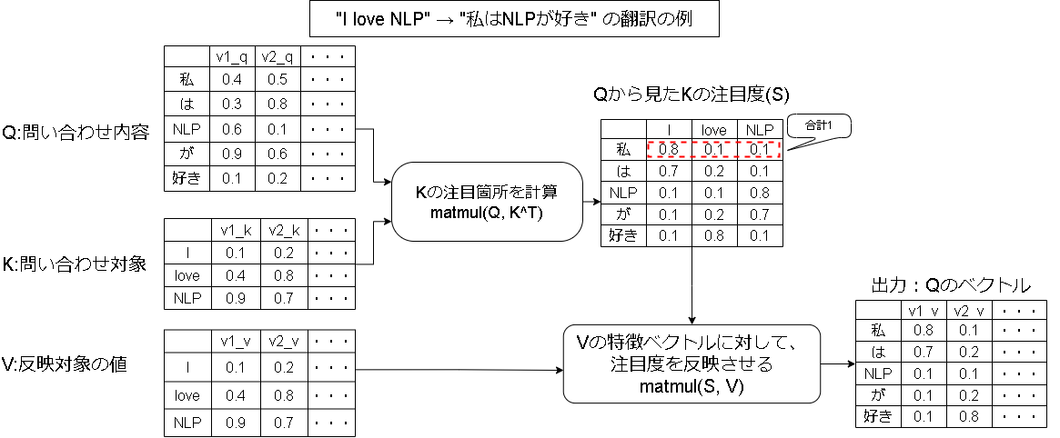
縦の列ですが、翻訳の例だとトークン列となりそのまま1次元で表現できますが、画像は2次元なのでw*hの1次元に並べ替えて表現させます。
(各ドットに対して別のドットに対する注目度を見るイメージ)
SelfAttentionは Q=K=V と、3つとも同じ値を入力したものになり、その画像内で関係性の高いドットを強調する役割になります。
説明は以上で、残りは実装結果です。
実行結果
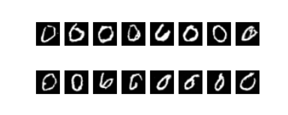
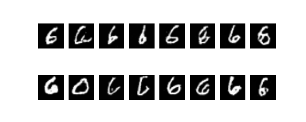
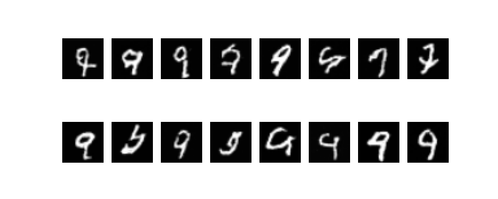
各数字を出力させてみました。
ちゃんとそれっぽい数字が出力されていますね。
ただモデルの大きさとlossの下がり具合的にまだ学習が足りていない気がします。
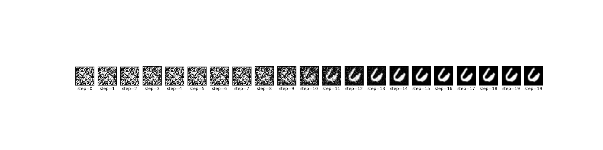
- 0
0のみhisotryものせておきます。
-
1

-
2

-
3

-
4

-
5

-
6
-
7

-
8

-
9
全体コード
version
- Windows11
- WSL2: Ubuntu24.04
- Python3.12.3
- Tensorflow 2.18.0
- CUDA 12.5.1
- cuDNN 9.3.0
- GeForce RTX 3060 12GB
import math
from functools import partial
from pathlib import Path

import numpy as np
import tensorflow as tf
from matplotlib import pyplot as plt
from tensorflow import keras
from tqdm import tqdm

kl = keras.layers


# define
img_size = 32
img_shape = (img_size, img_size, 1)


def create_dataset():
    (x_train, y_train), (_, _) = keras.datasets.mnist.load_data()
    # x_train, y_train = x_train[y_train == 1], y_train[y_train == 1]
    x_train = tf.image.resize(tf.expand_dims(x_train, -1), [img_size, img_size]).numpy()  # 28 -> 32
    x_train = (x_train / 255.0) * 2 - 1  # [0,255] -> [-1,1]
    return x_train.astype(np.float32), y_train.astype(np.float32)


def decode_image(x):
    img = np.clip(x, -1.0, 1.0)
    # [-1,1] -> [0,255]
    img = (((img + 1) / 2) * 255).astype(np.uint8)
    return img


# ----------------------------------
# model
# ----------------------------------

# alias
Conv2D1x1 = partial(kl.Conv2D, kernel_size=1, strides=1, padding="valid")
Conv2D3x3 = partial(kl.Conv2D, kernel_size=3, strides=1, padding="same")
IdentityLayer = partial(kl.Lambda, function=lambda x: x)  # 何もしないレイヤー


class PositionalEmbedding(keras.layers.Layer):
    def __init__(self, dim: int, **kwargs):
        super().__init__(**kwargs)
        self.dim = dim

    def call(self, time: tf.Tensor) -> tf.Tensor:
        half_dim = self.dim // 2
        embeddings = math.log(10000) / (half_dim - 1)
        embeddings = tf.exp(tf.range(half_dim, dtype=tf.float32) * -embeddings)
        embeddings = tf.expand_dims(time, axis=-1) * tf.expand_dims(embeddings, axis=0)
        embeddings = tf.concat([tf.math.sin(embeddings), tf.math.cos(embeddings)], axis=-1)
        return embeddings

    @staticmethod
    def plot(embedding_dim: int = 500, N: int = 100):  # for debug
        model = PositionalEmbedding(embedding_dim)
        timestep = EDM.create_timesptes(N)
        emb = model(tf.constant(timestep)).numpy()
        plt.pcolormesh(emb.T, cmap="RdBu")
        plt.ylabel("dimension")
        plt.xlabel("time step")
        plt.colorbar()
        plt.show()


class AdaGroupNorm(keras.layers.Layer):
    def __init__(self, group_size: int = 32, eps: float = 1e-5, **kwargs) -> None:
        super().__init__(**kwargs)
        self.group_size = group_size
        self.eps = eps

    def build(self, input_shape):
        in_channels = input_shape[-1]

        # group_sizeは割り切れる場合のみ指定、-1: LayerNorm, 1: InstanceNorm
        groups = self.group_size if in_channels % self.group_size == 0 else -1

        self.norm = kl.GroupNormalization(groups=groups, epsilon=self.eps)
        self.gamma = kl.Dense(in_channels, use_bias=False, kernel_initializer="zeros")
        self.beta = kl.Dense(in_channels, use_bias=False, kernel_initializer="zeros")

    def call(self, x, condition, training=False):
        x = self.norm(x, training=training)
        condition = tf.expand_dims(tf.expand_dims(condition, axis=1), axis=1)  # (b,c)->(b,1,1,c)
        gamma = self.gamma(condition, training=training)
        beta = self.beta(condition, training=training)
        return x * (1 + gamma) + beta


class SelfAttention2D(keras.layers.Layer):
    def __init__(self, head_dim: int = 8, **kwargs) -> None:
        super().__init__(**kwargs)
        self.head_dim = head_dim

    def build(self, input_shape):
        in_channels = input_shape[-1]
        self.n_head = max(1, in_channels // self.head_dim)
        assert in_channels % self.n_head == 0, f"入力チャンネル数はhead数で分割できる数(head={self.n_head})"
        self.norm = kl.GroupNormalization()
        self.qkv_proj = Conv2D1x1(in_channels * 3)
        self.out_proj = Conv2D1x1(in_channels, kernel_initializer="zeros", bias_initializer="zeros")
        self.softmax = kl.Softmax(axis=-1)

    def call(self, x, training=False):
        n, h, w, c = x.shape
        x = self.norm(x, training=training)
        qkv = self.qkv_proj(x)
        # chをヘッド数で分割、hとwはまとめてseq_lenとする
        # [batch, h, w, ch*3] -> [batch, h*w, ch//head, head*3]
        qkv = tf.reshape(qkv, (n, h * w, c // self.n_head, self.n_head * 3))
        # [batch, seq_len, head, d*3] -> [batch, head, seq_len, d*3]
        qkv = tf.transpose(qkv, perm=[0, 2, 1, 3])
        # -> [batch, head, seq_len, d] * 3
        q, k, v = tf.split(qkv, num_or_size_splits=3, axis=-1)
        attn = tf.matmul(q, k, transpose_b=True)  # q@k.T
        attn = attn / tf.math.sqrt(tf.cast(k.shape[-1], tf.float32))
        attn = tf.matmul(self.softmax(attn), v)
        # ヘッドを結合し、seq_len->h,wに分割
        # [batch, head, seq_len, d] -> [batch, seq_len, head, d] -> [batch, h, w, head*d]
        y = tf.transpose(attn, perm=[0, 2, 1, 3])
        y = tf.reshape(y, (n, h, w, c))
        return x + self.out_proj(y)


class Downsample(keras.layers.Layer):
    def build(self, input_shape):
        self.conv = kl.Conv2D(
            filters=input_shape[-1],
            kernel_size=3,
            strides=2,
            padding="same",
            kernel_initializer=keras.initializers.Orthogonal(),
        )

    def call(self, x, training=False):
        return self.conv(x, training=training)


class Upsample(keras.layers.Layer):
    def build(self, input_shape):
        self.conv = kl.Conv2D(
            filters=input_shape[-1],
            kernel_size=3,
            strides=1,
            padding="same",
        )

    def call(self, x, training=False):
        # 最近傍補間で2倍にリサイズ
        input_shape = tf.shape(x)
        x = tf.image.resize(x, size=(input_shape[1] * 2, input_shape[2] * 2), method="nearest")
        return self.conv(x, training=training)


class ResBlock(keras.Model):
    def __init__(self, channels: int, use_attention: bool, **kwargs) -> None:
        super().__init__(**kwargs)
        self.channels = channels
        self.use_attention = use_attention

    def build(self, input_shape):
        use_projection = input_shape[-1] != self.channels
        self.proj = Conv2D1x1(self.channels) if use_projection else IdentityLayer()
        self.norm1 = AdaGroupNorm()
        self.act1 = kl.Activation("silu")
        self.conv1 = Conv2D3x3(self.channels)
        self.norm2 = AdaGroupNorm()
        self.act2 = kl.Activation("silu")
        self.conv2 = Conv2D3x3(self.channels)
        self.attn = SelfAttention2D() if self.use_attention else IdentityLayer()

    def call(self, x, condition, training=False):
        r = self.proj(x, training=training)
        x = self.norm1(x, condition, training=training)
        x = self.act1(x, training=training)
        x = self.conv1(x, training=training)
        x = self.norm2(x, condition, training=training)
        x = self.act2(x, training=training)
        x = self.conv2(x, training=training)
        x = x + r
        x = self.attn(x, training=training)
        return x


class ResBlocks(keras.Model):
    def __init__(self, channels_list: list[int], use_attention: bool, **kwargs) -> None:
        super().__init__(**kwargs)
        self.resblocks = [ResBlock(c, use_attention) for c in channels_list]

    def call(self, x, condition=None, shortcut=None, training=False):
        outputs = []
        for i, resblock in enumerate(self.resblocks):
            if shortcut is not None:
                x = tf.concat([x, shortcut[i]], axis=-1)
            x = resblock(x, condition, training=training)
            outputs.append(x)
        return x, outputs


class UNet(keras.Model):
    def __init__(self, img_shape: tuple, category_num: int, **kwargs) -> None:
        super().__init__(**kwargs)

        # condition
        embedding_dim = 128
        self.time_embedding1 = PositionalEmbedding(embedding_dim)
        self.time_embedding2 = kl.Dense(embedding_dim, activation="gelu")
        self.time_embedding3 = kl.Dense(embedding_dim)
        self.category_embedding1 = kl.Embedding(category_num, embedding_dim)
        self.category_embedding2 = kl.Dense(embedding_dim, activation="gelu")
        self.category_embedding3 = kl.Dense(embedding_dim)

        # Note: SelfAttentionは画像サイズが大きい場合に適用するとメモリ不足になった

        # downsample
        self.down_block11 = ResBlocks([32, 32], use_attention=False)
        self.down_block12 = ResBlocks([32, 32], use_attention=False)
        self.down_block13 = ResBlocks([32, 32], use_attention=False)
        self.downsample1 = Downsample()
        self.down_block21 = ResBlocks([32, 32], use_attention=False)
        self.down_block22 = ResBlocks([32, 32], use_attention=False)
        self.down_block23 = ResBlocks([32, 32], use_attention=False)
        self.downsample2 = Downsample()

        # middle
        self.middle_block = ResBlocks([256], use_attention=True)

        # upsample
        self.up_block23 = ResBlocks([32, 32], use_attention=False)
        self.up_block22 = ResBlocks([32, 32], use_attention=False)
        self.up_block21 = ResBlocks([32, 32], use_attention=False)
        self.upsample2 = Upsample()
        self.up_block13 = ResBlocks([32, 32], use_attention=False)
        self.up_block12 = ResBlocks([32, 32], use_attention=False)
        self.up_block11 = ResBlocks([32, 32], use_attention=False)
        self.upsample1 = Upsample()

        # 出力層(正規分布のノイズ画像)
        self.out_layer = kl.Conv2D(1, (1, 1), padding="same")

        # build & init weight
        self(
            [
                np.zeros((1,) + img_shape),
                np.zeros((1,)),
                np.zeros((1,)),
            ]
        )

    @tf.function
    def call(self, inputs, training=False):
        # 入力: (ノイズ画像、時間ステップ、カテゴリ)
        x, t, category = inputs

        # 時間埋め込み
        t_emb = self.time_embedding1(t, training=training)
        t_emb = self.time_embedding2(t_emb, training=training)
        t_emb = self.time_embedding3(t_emb, training=training)

        # カテゴリの埋め込み
        c_emb = self.category_embedding1(category, training=training)
        c_emb = self.category_embedding2(c_emb, training=training)
        c_emb = self.category_embedding3(c_emb, training=training)

        # 条件付けはtimesteps+catetory
        condition = t_emb + c_emb

        # --- U-Net
        x, o11 = self.down_block11(x, condition, training=training)
        x, o12 = self.down_block12(x, condition, training=training)
        x, o13 = self.down_block13(x, condition, training=training)
        x = self.downsample1(x, training=training)  # 28x28 -> 14x14
        x, o21 = self.down_block21(x, condition, training=training)
        x, o22 = self.down_block22(x, condition, training=training)
        x, o23 = self.down_block23(x, condition, training=training)
        x = self.downsample2(x, training=training)  # 14x14 -> 7x7

        x, _ = self.middle_block(x, condition, training=training)

        x = self.upsample2(x, training=training)  # 7x7 -> 14x14
        x, _ = self.up_block23(x, condition, o23[::-1], training=training)
        x, _ = self.up_block22(x, condition, o22[::-1], training=training)
        x, _ = self.up_block21(x, condition, o21[::-1], training=training)
        x = self.upsample1(x, training=training)  # 14x14 -> 28x28
        x, _ = self.up_block13(x, condition, o13[::-1], training=training)
        x, _ = self.up_block12(x, condition, o12[::-1], training=training)
        x, _ = self.up_block11(x, condition, o11[::-1], training=training)

        x = self.out_layer(x, training=training)
        return x


class EDM:
    def __init__(self, img_shape, category_num, lr: float = 0.0001, sigma_data=0.5):
        self.sigma_data = sigma_data
        self.model = UNet(img_shape, category_num)
        self.optimizer = keras.optimizers.Adam(learning_rate=lr)

    def calc_c(self, sigma):
        c_skip = self.sigma_data**2 / (sigma**2 + self.sigma_data**2)
        c_out = sigma * self.sigma_data / tf.sqrt(sigma**2 + self.sigma_data**2)
        c_in = 1 / tf.sqrt(self.sigma_data**2 + sigma**2)
        c_noise = tf.math.log(sigma) / 4
        return c_skip, c_out, c_in, c_noise

    def call(self, x, sigma, category, training=False):
        c_skip, c_out, c_in, c_noise = self.calc_c(sigma)
        c_noise = tf.reshape(c_noise, (-1,))
        fx = self.model([c_in * x, c_noise, category], training=training)
        dx = c_skip * x + c_out * fx
        return dx

    def train(self, img, category, p_mean=-1.2, p_std=1.2):
        # Noise distibution: ln(σ) ~ N(Pmena, Pstd^2)
        r = np.random.randn(img.shape[0], 1, 1, 1).astype(np.float32)
        sigma = np.exp(p_mean + r * p_std)
        c_skip, c_out, c_in, c_noise = self.calc_c(sigma)
        c_noise = tf.reshape(c_noise, (-1,))

        # λ(σ): (σ^2+σd^2) / (σ*σd)^2
        lambda_w = (sigma**2 + self.sigma_data**2) / ((sigma * self.sigma_data) ** 2)

        # ノイズ
        n = np.random.randn(*img.shape) * sigma

        # tensorflowに取り込める形に変換
        n = tf.convert_to_tensor(n, dtype=tf.float32)
        sigma = tf.convert_to_tensor(sigma.reshape((-1, 1, 1, 1)), dtype=tf.float32)

        with tf.GradientTape() as tape:
            output = self.model([c_in * (img + n), c_noise, category])
            target = (img - c_skip * (img + n)) / c_out
            loss = lambda_w * (c_out**2) * ((output - target) ** 2)
            loss = tf.reduce_mean(loss)
        grad = tape.gradient(loss, self.model.trainable_variables)
        self.optimizer.apply_gradients(zip(grad, self.model.trainable_variables))

        return loss.numpy()

    def generate(
        self,
        size: int,
        N: int,
        category: int,
        sigma_min=0.002,
        sigma_max=80,
        rho=7,
        s_churn=0,
        s_min=0,
        s_max=float("inf"),
        s_noise=1,
    ):
        # Time steps
        timesteps = self.create_timesptes(N, sigma_min, sigma_max, rho)
        tf_category = tf.convert_to_tensor([category] * size, dtype=tf.float32)

        samples_history = []

        # 初期サンプル
        var = timesteps[0]
        x = np.random.randn(size, *img_shape).astype(np.float32) * var

        x = tf.convert_to_tensor(x, dtype=tf.float32)
        for t, next_t in tqdm(
            zip(timesteps[:-1], timesteps[1:]),
            total=N,
            desc="sampling loop",
        ):
            gamma = min(s_churn / N, np.sqrt(2) - 1) if s_min <= t <= s_max else 0
            t_hat = t + gamma * t
            e = np.random.randn(size, *img_shape).astype(np.float32) * s_noise
            x_hat = x + np.sqrt(t_hat**2 - t**2) * e

            # tf
            t_hat = tf.convert_to_tensor([t_hat] * size, dtype=tf.float32)
            t_hat = tf.reshape(t_hat, (-1, 1, 1, 1))
            denoise = self.call(x_hat, t_hat, tf_category)

            d = (x_hat - denoise) / t_hat
            x_next = x_hat + (next_t - t_hat) * d
            if next_t != 0:
                # tf
                t_next = tf.convert_to_tensor([next_t] * size, dtype=tf.float32)
                t_next = tf.reshape(t_next, (-1, 1, 1, 1))
                denoise = self.call(x_next, t_next, tf_category)

                d_dash = (x_next - denoise) / next_t
                x_next = x_hat + (next_t - t_hat) * (d / 2 + d_dash / 2)

            samples_history.append(x_next)
            x = x_next

        return x, samples_history

    @staticmethod
    def create_timesptes(N: int, sigma_min=0.002, sigma_max=80, rho=7):
        timesteps = []
        for i in range(N):
            t = (sigma_max ** (1 / rho) + i / (N - 1) * (sigma_min ** (1 / rho) - sigma_max ** (1 / rho))) ** rho
            timesteps.append(t)
        timesteps += [0]  # N=0
        return timesteps


# ----------------------------------
# main
# ----------------------------------
def plot_summary():
    # U-Net
    model = UNet(img_shape, category_num=10)
    model.summary()

    # Time steps
    timesptes = EDM.create_timesptes(20)
    plt.figure(figsize=(8, 5))
    plt.plot(range(len(timesptes)), timesptes, marker=".")
    plt.xlabel("i")
    plt.ylabel("Time step")
    plt.title("Visualization of Time steps")
    plt.grid()
    plt.show()

    # 位置エンコーディングの可視化
    PositionalEmbedding.plot()


def train(epochs: int, batch_size: int, lr: float):
    x_img, x_category = create_dataset()

    # モデル
    edm = EDM(img_shape, category_num=10, lr=lr)

    # 学習用にデータをバッチ化
    train_dataset = tf.data.Dataset.from_tensor_slices((x_img, x_category)).shuffle(len(x_img)).batch(batch_size)

    for epoch in range(epochs):
        with tqdm(train_dataset, desc=f"Epoch {epoch + 1}/{epochs}") as pbar:
            for img, category in pbar:
                loss = edm.train(img, category)
                pbar.set_postfix(loss=loss)  # 損失を進捗バーに表示
    edm.model.save_weights(Path(__file__).parent / "edm.weights.h5")


def generate(steps: int, category: int, **gen_kwargs):
    edm = EDM(img_shape, category_num=10)
    edm.model.load_weights(Path(__file__).parent / "edm.weights.h5")

    # 生成
    num_w = 8
    num_h = 2
    num_samples = num_w * num_h
    samples, samples_history = edm.generate(num_samples, steps, category, **gen_kwargs)

    samples = decode_image(samples)
    samples_history = decode_image(samples_history)

    # 結果
    plt.figure(figsize=(10, 4))
    for i in range(num_samples):
        plt.subplot(num_h, num_w, i + 1)
        plt.imshow(samples[i, :, :, 0], cmap="gray")
        plt.axis("off")
    plt.savefig(Path(__file__).parent / f"plot_{category}.png")
    # plt.show()

    # 作成過程
    index = 4
    img_list = np.array(samples_history)[:, index, :, :, 0]
    plt.figure(figsize=(20, 5))
    step_idxs = list(range(0, len(img_list), int(steps / 12)))  # 多いので一定間隔で抜き出し
    step_idxs += [len(img_list) - 1]  # 最後も追加
    for i, idx in enumerate(step_idxs):
        plt.subplot(1, len(step_idxs), i + 1)
        plt.imshow(img_list[idx], cmap="gray")
        plt.xticks([])
        plt.yticks([])
        plt.xlabel(f"step={idx}")
    plt.savefig(Path(__file__).parent / f"plot_{category}_history.png")
    # plt.show()


if __name__ == "__main__":
    # plot_summary()
    train(epochs=10, batch_size=128, lr=0.0002)
    for i in range(10):
        generate(steps=20, category=i)
モデルのsummary
TFは2階層以上のクラスのshapeがデフォルトで表示されません。(昔から解決策を調べてるんですが…、分かる方教えてください)
Model: "u_net"
┏━━━━━━━━━━━━━━━━━━━━━━━━━━━━━━━━━━━━━━┳━━━━━━━━━━━━━━━━━━━━━━━━━━━━━┳━━━━━━━━━━━━━━━━━┓
┃ Layer (type)                         ┃ Output Shape                ┃         Param # ┃
┡━━━━━━━━━━━━━━━━━━━━━━━━━━━━━━━━━━━━━━╇━━━━━━━━━━━━━━━━━━━━━━━━━━━━━╇━━━━━━━━━━━━━━━━━┩
│ positional_embedding                 │ ?                           │               0 │
│ (PositionalEmbedding)                │                             │                 │
├──────────────────────────────────────┼─────────────────────────────┼─────────────────┤
│ dense (Dense)                        │ (1, 128)                    │          16,512 │
├──────────────────────────────────────┼─────────────────────────────┼─────────────────┤
│ dense_1 (Dense)                      │ (1, 128)                    │          16,512 │
├──────────────────────────────────────┼─────────────────────────────┼─────────────────┤
│ embedding (Embedding)                │ (1, 128)                    │           1,280 │
├──────────────────────────────────────┼─────────────────────────────┼─────────────────┤
│ res_blocks (ResBlocks)               │ ?                           │          53,154 │
├──────────────────────────────────────┼─────────────────────────────┼─────────────────┤
│ res_blocks_1 (ResBlocks)             │ ?                           │          70,016 │
├──────────────────────────────────────┼─────────────────────────────┼─────────────────┤
│ downsample (Downsample)              │ ?                           │           9,248 │
├──────────────────────────────────────┼─────────────────────────────┼─────────────────┤
│ res_blocks_2 (ResBlocks)             │ ?                           │          70,016 │
├──────────────────────────────────────┼─────────────────────────────┼─────────────────┤
│ res_blocks_3 (ResBlocks)             │ ?                           │          70,016 │
├──────────────────────────────────────┼─────────────────────────────┼─────────────────┤
│ downsample_1 (Downsample)            │ ?                           │           9,248 │
├──────────────────────────────────────┼─────────────────────────────┼─────────────────┤
│ res_blocks_4 (ResBlocks)             │ ?                           │         296,384 │
├──────────────────────────────────────┼─────────────────────────────┼─────────────────┤
│ res_blocks_5 (ResBlocks)             │ ?                           │         164,608 │
├──────────────────────────────────────┼─────────────────────────────┼─────────────────┤
│ res_blocks_6 (ResBlocks)             │ ?                           │         109,120 │
├──────────────────────────────────────┼─────────────────────────────┼─────────────────┤
│ upsample (Upsample)                  │ ?                           │         147,584 │
├──────────────────────────────────────┼─────────────────────────────┼─────────────────┤
│ res_blocks_7 (ResBlocks)             │ ?                           │         109,120 │
├──────────────────────────────────────┼─────────────────────────────┼─────────────────┤
│ res_blocks_8 (ResBlocks)             │ ?                           │         109,120 │
├──────────────────────────────────────┼─────────────────────────────┼─────────────────┤
│ upsample_1 (Upsample)                │ ?                           │           9,248 │
├──────────────────────────────────────┼─────────────────────────────┼─────────────────┤
│ conv2d (Conv2D)                      │ (1, 32, 32, 1)              │              33 │
└──────────────────────────────────────┴─────────────────────────────┴─────────────────┘
 Total params: 1,261,219 (4.81 MB)
 Trainable params: 1,261,219 (4.81 MB)
 Non-trainable params: 0 (0.00 B)
学習途中のloss
Epoch 1/10: 100%|███████████████████| 469/469 [09:29<00:00,  4.22s/it, loss=0.178]
Epoch 1/10: 100%|███████████████████| 469/469 [09:29<00:00,  1.21s/it, loss=0.178]
Epoch 2/10: 100%|███████████████████| 469/469 [08:44<00:00,  1.10s/it, loss=0.153]
Epoch 2/10: 100%|███████████████████| 469/469 [08:44<00:00,  1.12s/it, loss=0.153]
Epoch 3/10: 100%|███████████████████| 469/469 [08:15<00:00,  1.06s/it, loss=0.147]
Epoch 4/10: 100%|███████████████████| 469/469 [08:02<00:00,  1.03s/it, loss=0.119]
Epoch 4/10: 100%|███████████████████| 469/469 [08:02<00:00,  1.03s/it, loss=0.119]
Epoch 5/10: 100%|███████████████████| 469/469 [07:27<00:00,  1.05it/s, loss=0.128]
Epoch 6/10: 100%|███████████████████| 469/469 [07:15<00:00,  1.08it/s, loss=0.113]
Epoch 7/10: 100%|███████████████████| 469/469 [07:13<00:00,  1.08it/s, loss=0.104]
Epoch 8/10: 100%|███████████████████| 469/469 [07:17<00:00,  1.01it/s, loss=0.113]
Epoch 8/10: 100%|███████████████████| 469/469 [07:17<00:00,  1.07it/s, loss=0.113]
Epoch 9/10: 100%|███████████████████| 469/469 [07:07<00:00,  1.10it/s, loss=0.115]
Epoch 10/10: 100%|██████████████████| 469/469 [07:12<00:00,  1.08it/s, loss=0.12]
おわりに
これで拡散モデルは終わりな気がする(多分→つd)
学習が少ないと前の小さいモデルの方がすぐ学習できて優秀に感じました。
このモデルもパラメータ数をもっと増やして長時間学習させれば精度が上がりそうな感じはしています。
後、学習率を徐々に下げていった方がいいかも。
誰かの参考になれば幸いです。