メルカリのkaggleコンペデータ分析に初心者が挑戦してみる

【自己紹介】

社会人3年目、完全な文系出身です。
1年ほどゆるゆると独学でプログラミングを学習し、
直近3か月間、Aidemyさんでスクールを受講しました。

本ブログの内容が初めてのデータ分析実践となります。
まずは自分が興味を持てる内容として、
実際に使用しているメルカリのコンペデータを分析してみました。

【使用するデータについて】

Mercari Price Suggestion Challenge

今回の分析で使用するデータは、コンペサイトkaggleで提供されている
フリマアプリmercariの商品情報データです。

本コンペでは、テストデータに含まれる商品の
販売価格を予想することが分析の目的となっています。

【本分析の目的】

今回の分析では、Aidemyで学習した内容を一通り試しながら、
作成したモデルの精度改善を図っていくことを目的としています。

【分析の流れ】

・データ観察
・データ前処理
・モデル作成
・スコア確認
・データ再処理
・再度モデル作成
・スコア確認

【データ観察】

○データの概要

データを読み込み、"price"をターゲットに、
そしてtrainとtestを結合してフラグを付けておきます。

train_df = pd.read_csv('/content/drive/MyDrive/datasets/mercari/mercari_train.tsv', delimiter='\t')
test_df = pd.read_csv('/content/drive/MyDrive/datasets/mercari/mercari_test.tsv', delimiter='\t')

train_df = train_df.rename(columns = {"train_id":"id"})
test_df = test_df.rename(columns = {"test_id":"id"})
target = train_df["price"]

all_df = pd.concat([train_df.drop(["price"], axis=1), test_df],axis=0).reset_index(drop=True)
all_df['Test_Flag'] = 0
all_df.loc[train_df.shape[0]: , 'Test_Flag'] = 1

まずは読み込んだデータを確認します。

print(train_df.shape)
print(test_df.shape)

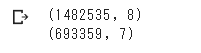
各columnの詳細は以下の通りです。
・train_id or test_id / 各商品投稿についたID。
・name / 各投稿のタイトル。nameに価格が含まれていた場合は[rm]で修正。
　　 　例）”食パン 30$ 限界価格” → “食パン [rm] 限界価格”
・item_condition_id / 出品者が提供する商品の状態。
・category_name / 投稿商品のカテゴリー。
・brand_name / 投稿商品のブランド名。
・price / 最終的に取引された価格。本コンペのターゲット。train限定。
・shipping / 送料を出品者が負担の場合は1、買い手が負担の場合は0
・item_description / 商品説明の全文。nameと同様価格の表記は[rm]に修正。

train_df.head()

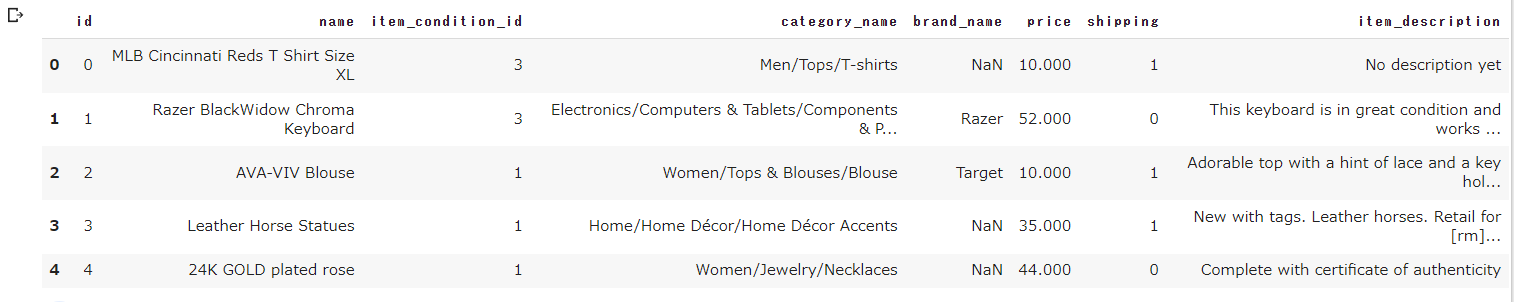
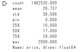
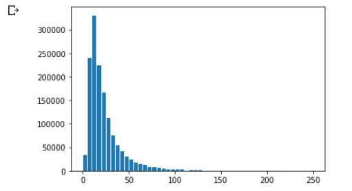
○“price”について

価格は最低が0＄、最大が2009＄、
全体的に小さい方に偏ったデータになっています。

target.describe()

import matplotlib.pyplot as plt
plt.hist(train_df["price"],bins=50, edgecolor='white', range=[0, 250])
plt.show()

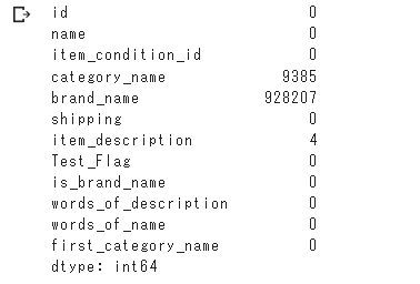
○欠損値の確認

欠損値はcategory_nameとbrand_nameの中で多く見られます。

all_df.isnull().sum()

○現時点での考察

各columnについて、価格に対する影響の仕方を考えてみる。
・name / 何の商品か説明する項目なので最重要。
　　　 　最初の分析ではnameに含まれる単語量(どれだけ説明されているか)で処理。
・item_condition_id / 新品の方が高くなる傾向はあるが、重要度は低め。
・category_name / 投稿の必須項目ではないため、重要度は低め。
・brand_name / ブランド毎にある程度の価格帯があると予想されるため、重要度は中。
・shipping / 送料込(出品者負担)の方が販売価格は高くなるが、重要度は低め。
・item_description / こちらも最重要。nameと同様に処理。

○分析手法について

今回は連続した数値の予測ということなので、
Lasso、Ridge、ElasticNetを使ってみることにしました。

一度簡単な処理で精度を出して確認し、
その後処理の方法を変えて精度の変化を確認します。

【データ前処理：1回目】

○欠損値の確認

欠損は以下の2項目に見られる。
・brand_name
・category_name
上記についてはこの後、欠損値の処理を含めつつ、
数値に変換していく作業を行っていきます。

○nameとitem_descriptionの処理

最初手をつけた時、自然言語を扱うのはなんとなく
難しく感じたため、とりあえず単語量のみを数値に変換しました。
(詳細を書けば書くほど価格が上がるという安直な予想)

#item_description：文章量に含まれる単語数をカウント
def words_count_description(text):
  if text == "No description yet":
    return 0
  else:
    return len(str(text).split())

all_df["words_of_description"] = all_df["item_description"].map(words_count_description)

#name：含まれる単語量をカウント
def words_count_name(text):
  if text == "NaN":
    return 0
  else:
    return len(str(text).split())

all_df["words_of_name"] = all_df["name"].map(words_count_name)

○brand_nameの処理

まずはシンプルにブランドの登録がある場合は1、
ない場合は0として処理を行なった。

#brand_name：ある場合は1、ない場合は0に変換
all_df["is_brand_name"] = np.where(all_df["brand_name"].isnull(),0,1)

〇category_nameの処理

こちらはcategoryを詳細に分けると特徴量が多かったので、
とりあえず各categoryの最上位のジャンルのみ抽出する処理を行なった。
例)men > tops > shirts の場合は「men」を抽出

#category_name：カテゴリ最初の単語を抽出
def pick_first_category(text):
  if text == False:
    return "NaN"
  else:
    return str(text).split("/")[0]

all_df["first_category_name"] = all_df["category_name"].map(pick_first_category)

#カテゴリー名を数値にエンコード
Encode_category_list = all_df["first_category_name"].unique().tolist()

def encode_category(ctg):
  return Encode_category_list.index(ctg)

all_df["first_category_name"] = all_df["first_category_name"].map(encode_category)

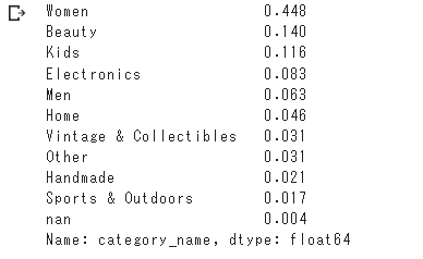
ちなみに各最上位カテゴリーの割合は以下の通り。
女性向けの商品が半数近く占めてます。

all_df["category_name"].map(pick_first_category).value_counts(normalize=True)

〇trainデータとtestデータを分離

上記の処理によって、全ての特徴量を数値に変換することができたため、
モデルの作成に向けてデータをtrainとtestに戻しておく。

#不要な特徴量を削除したdataframeを作成
all_df_for_model = all_df[['id', 'item_condition_id', 'shipping', 'Test_Flag', 'is_brand_name',
       'words_of_description', 'words_of_name', 'first_category_name']]

#念のためint型に変換
all_df_for_model = all_df_for_model.astype(int)

#train,test用のドロップカラム
drop_col = ["id", "Test_Flag"]

test = all_df_for_model.loc[all_df_for_model["Test_Flag"]==1].drop(drop_col, axis=1).reset_index(drop=True)
train = all_df_for_model.loc[all_df_for_model["Test_Flag"]==0].drop(drop_col, axis=1)

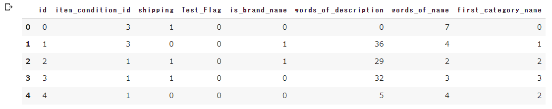
一応今の時点でデータフレームはこんな感じ。

all_df_for_model.head()

【モデル作成と学習：1回目】

前述の通り、まずはLasso、Ridge、ElasticNetで試しに作成。

学習のためにtrainデータの7割を使用し、
残りの3割はValidationデータとして精度評価に使用する。

from sklearn.model_selection import train_test_split
X_train, X_val, y_train, y_val = train_test_split(train, target, test_size=0.3)

from sklearn.linear_model import Lasso
model_Lasso = Lasso()
model_Lasso.fit(X_train, y_train)

print("Lasso")
print(f"train_score:{model_Lasso.score(X_train, y_train)}")
print(f"val_score:{model_Lasso.score(X_val, y_val)}")


from sklearn.linear_model import ElasticNet
model_Ela = ElasticNet()
model_Ela.fit(X_train, y_train)

print("")
print("ElasticNet")
print(f"train_score:{model_Ela.score(X_train, y_train)}")
print(f"val_score:{model_Ela.score(X_val, y_val)}")


from sklearn.linear_model import Ridge
model_Ridge = Ridge()
model_Ridge.fit(X_train, y_train)

print("")
print("Ridge")
print(f"train_score:{model_Ridge.score(X_train, y_train)}")
print(f"val_score:{model_Ridge.score(X_val, y_val)}")

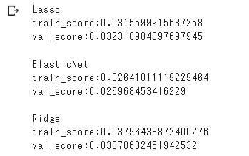
最もスコアの高いRidgeモデルでも4%弱という悲しい結果であった。
3つのモデルの中ではRidge回帰が最もスコアが高かったため、
次の試行ではRidge回帰でのスコア改善を図る。

○ここまでの考察

やはり価格を決める要素として、検索の対象となる
・name
・item_description
の処理に一番の課題があると考えた。

次の段階では、文章や含まれる単語の意味も
考慮した状態での処理を行うこととした。

【データ前処理：2回目】

〇priceの処理

本コンペの評価指標はRMSLE(対数平均二乗誤差)というもので、
対数を取ったでの誤差を計算必要があるとのこと。
なので先にpriceをnp.log1pで処理しておく。

target = np.log1p(train_df["price"].values)

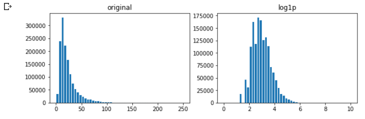
ちなみにpriceのlogを取った状態でヒストグラムを見ると、
グラフの形がこんな風に変換される。

import matplotlib.pyplot as plt
fig = plt.figure(figsize = (10,3))

#画像左側
ax1 = fig.add_subplot(121)
ax1.set_title("original")
ax1.hist(train_df["price"], bins=50, edgecolor='white', range=[0, 250])

#画像右側
ax2 = fig.add_subplot(122)
ax2.set_title("log1p")
ax2.hist(target, bins=50, edgecolor='white', range=[0, 10])
plt.show()

〇欠損値の処理

1回目の処理では他の作業に含めていたが、
今回は事前にまとめて以下の処理を行う。

#欠損値を処理
all_df["category_name"].fillna("NaN", inplace=True)
all_df["brand_name"].fillna("None", inplace=True)
all_df["item_description"].fillna("No description yet", inplace=True)

○brand_nameの処理

ブランドの登録数が多ければ、そのブランドの価格帯が大まかに分かり、
価格予測に役立つと考え、以下の処理を行うことにした。

#ブランド上位300個のみ抽出、それ以外はNoneに変換
drop_brand_list = all_df["brand_name"].value_counts().index[300:]

def drop_brand(brand):
  if brand in drop_brand_list:
    return "None"
  else:
    return brand

all_df["brand_name"] = all_df["brand_name"].map(drop_brand)

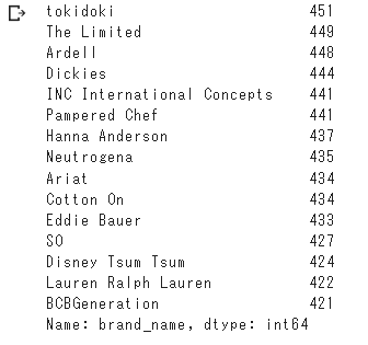
value_countsで数の多い方から上位300個のブランドを抽出。
上位300個に含まれないブランドのデータは、“None”に変換を行なった。

変換後、件数の下位15ブランドは以下の通りとなっており、
最低でも400件以上投稿されているブランドに絞られた。

all_df["brand_name"].value_counts()[-15:]

○自然言語処理の活用

・name
・item_description
上記2点について自然言語処理で学んだ内容を適用してみることにした。

nameは単語をメインとした簡単な文章のため、
CountVectorizerを使用して、ベクトル変換を行う。

item_descriptionはnameよりも文章としての意味合いが強いため、
TfidfVectorizerを使用する。

count_name = CountVectorizer(min_df=10)
X_name = count_name.fit_transform(all_df["name"])

tfidf_description = TfidfVectorizer(max_features = 200, stop_words = "english", ngram_range = (1,3))
X_description = tfidf_description.fit_transform(all_df["item_description"])

最初nameもtf-idfで試したが試行の結果、
最終的にCountVectorizerの方がスコアは高くなった。

nameをTfidfVectorizerで変換して学習した時
train_score:0.1463342867889036
val_score:0.14966227842923285

原因としてはやはり、
名前と説明で分の構成が大きく変わり、
単語の持つ影響力に差があったためかと思われる。

○category_nameの処理

前回は各カテゴリーの最上位を抽出したが、
今回は各カテゴリーの最下位を抽出し、より詳細な分類を行う。
例)men > tops > shirts の場合は「shirts」を抽出

def pick_last_category(text):
  if text == "NaN":
    return "NaN"
  else:
    return str(text).split("/")[-1]

all_df["last_category_name"] = all_df["category_name"].map(pick_last_category)

○ダミー変数化

・item_condition_id
・shipping
・brand_name
・last_category_name
こちらの4点に関しては、
pandasのget_dummiesを使用し、ダミー変数化を行う。
引数にsparse=Trueとして、疎行列で出力を行う。

#get_dummiesを使用するため、カテゴリー型に変換
all_df["brand_name"] = all_df["brand_name"].astype("category")
all_df["item_condition_id"] = all_df["item_condition_id"].astype("category")
all_df["shipping"] = all_df["shipping"].astype("category")

import scipy
X_dummies = scipy.sparse.csr_matrix(pd.get_dummies(all_df[["item_condition_id", "shipping", "last_category_name", "brand_name"]], sparse = True).values)

○各列の結合

scipyのsparse.hstackを使用し、全ての要素を結合する。
そのデータを元のtrainとtestに分割し、
後は1回目と同様にモデル作成、学習を行える状態となった。

X = scipy.sparse.hstack((X_name , X_description, X_dummies)).tocsr()

shape = train_df.shape[0]
train = X[:shape]
test = X[shape:]

X_train, X_val, y_train, y_val = train_test_split(train, target, test_size=0.3)

【モデル作成と学習：2回目】

今回はモデル作成に使用する特徴量がとても多く、
全ての特徴量が予測に重要になるため、
Ridge回帰での学習にて比較を行うこととした。

model_Ridge = Ridge()
model_Ridge.fit(X_train, y_train)

print(f"train_score:{model_Ridge.score(X_train, y_train)}")
print(f"val_score:{model_Ridge.score(X_val, y_val)}")

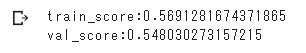
特にパラメータは設定せずに学習を行なったが、
前回と比べて大幅な改善となった。

○パラメータ「alpha」の調整

調べたらRidge回帰にはalphaというパラメータがあるのが分かったため、
最も精度が高まるalphaを一応調べてみた。

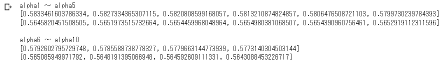
alpha = 1 〜 10で試行し、各結果をリストに格納。
trainとvalidationのスコアを描画し、
またtrainとvalidationの差分も同じように描画行う。

int_list = np.arange(1,11)
train_score = []
val_score = []

for i in int_list:

  model_Ridge = Ridge(alpha=i)
  model_Ridge.fit(X_train, y_train)
  train_score.append(model_Ridge.score(X_train, y_train))
  val_score.append(model_Ridge.score(X_val, y_val))

print("alpha1 ～ alpha5")
print(train_score[:6])
print(val_score[:6])

print("")
print("alpha6 ～ alpha10")
print(train_score[6:11])
print(val_score[6:11])

import matplotlib.pyplot as plt

dif_list = []
for train, val in zip(train_score, val_score):
  dif_list.append(train - val)

fig = plt.figure(figsize = (10,3))

ax1 = fig.add_subplot(121)
ax1.set_title("score")
ax1.plot(int_list, train_score, color="y", label="train")
ax1.plot(int_list, val_score, color="b", label="val")
ax1.legend()

ax2 = fig.add_subplot(122)
ax2.set_title("different_train_val")
ax2.plot(int_list, dif_list, color="r")

plt.show()

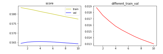
上のグラフからも、alpha=4 のときにvalidationに対する精度が高く、
alphaが大きいほど、trainとvalidationの誤差は小さくなることが分かった。
最終的なモデルの完成には、alpha=4とすることにした。

最後にモデルを再度作成し、
validationに対してのRMSLEを算出する。

model_Ridge = Ridge(alpha=4)
model_Ridge.fit(X_train, y_train)

y_pred = model_Ridge.predict(X_val)
RMSLE = np.sqrt(np.mean(np.square(y_pred - y_val)))
print(RMSLE)

今回作成したモデルでのRMSLEは0.4939程度であった。

本コンペで1stを取ったカーネルが0.3875であり、
実際の価格3,000円の場合、2,036円~4,420円程度の誤差範囲にある。

RRMSLEが0.4939だと、
実際の価格3,000円の場合、1,831円~4,916円程度の誤差範囲にある。
初めて分析したにしては、それなりの結果のようにも見える、かも知れない。

【サブミット】

最後は今までに作ったモデルでテストデータを予測して、
kaggleのweb上にてサブミットするためのデータを出力する。

test_pred = model_Ridge.predict(test)
sample_sub = pd.read_csv("/content/drive/MyDrive/datasets/mercari/sample_submission.csv")
sample_sub["price"] = np.expm1(test_pred)
sample_sub.to_csv("submission.csv", index=False)

【最後に】

今回のコードの全容は以下の通りです。

import pandas as pd
from IPython.display import display
from sklearn import metrics
from sklearn.model_selection import train_test_split
pd.set_option('display.float_format', lambda x:'%.3f' % x)
import numpy as np
from sklearn.linear_model import Ridge
from sklearn.model_selection import train_test_split
from sklearn.feature_extraction.text import CountVectorizer, TfidfVectorizer

train_df = pd.read_csv('/content/drive/MyDrive/datasets/mercari/mercari_train.tsv', delimiter='\t')
test_df = pd.read_csv('/content/drive/MyDrive/datasets/mercari/mercari_test.tsv', delimiter='\t')

all_df = pd.concat([train_df.drop(["price"], axis=1), test_df],axis=0).reset_index(drop=True)
target = np.log1p(train_df["price"].values)
shape = train_df.shape[0]

#欠損値を処理
all_df["category_name"].fillna("NaN", inplace=True)
all_df["brand_name"].fillna("None", inplace=True)
all_df["item_description"].fillna("No description yet", inplace=True)

#ブランド上位300個のみ抽出、それ以外はNoneに変換
drop_brand_list = all_df["brand_name"].value_counts().index[300:]

def drop_brand(brand):
  if brand in drop_brand_list:
    return "None"
  else:
    return brand

all_df["brand_name"] = all_df["brand_name"].map(drop_brand)

#後にget_dummiesを利用するため、カテゴリー型に変換
all_df["brand_name"] = all_df["brand_name"].astype("category")
all_df["item_condition_id"] = all_df["item_condition_id"].astype("category")
all_df["shipping"] = all_df["shipping"].astype("category")

count_name = CountVectorizer(min_df=10)
X_name = count_name.fit_transform(all_df["name"])

tfidf_description = TfidfVectorizer(max_features = 200, stop_words = "english", ngram_range = (1,3))
X_description = tfidf_description.fit_transform(all_df["item_description"])

#各カテゴリーの末端を単語抽出
def pick_last_category(text):
  if text == "NaN":
    return "NaN"
  else:
    return str(text).split("/")[-1]

all_df["last_category_name"] = all_df["category_name"].map(pick_last_category)

#4項目をダミー変数化、疎行列変換
import scipy
X_dummies = scipy.sparse.csr_matrix(pd.get_dummies(all_df[["item_condition_id", "shipping", "last_category_name", "brand_name"]], sparse = True).values)

#データを結合し、trainとtestに分割
X = scipy.sparse.hstack((X_name , X_description, X_dummies)).tocsr()

train = X[:shape]
test = X[shape:]
X_train, X_val, y_train, y_val = train_test_split(train, target, test_size=0.3)

#モデル作成、学習の後、submitファイルを出力
model_Ridge = Ridge(alpha=4)
model_Ridge.fit(X_train, y_train)

test_pred = model_Ridge.predict(test)
sample_sub = pd.read_csv("/content/drive/MyDrive/datasets/mercari/sample_submission.csv")
sample_sub["price"] = np.expm1(test_pred)
sample_sub.to_csv("submission.csv", index=False)

初めて学習用以外のデータに触れて、
本当に色々なところで躓きがありました。

nameとdescriptionについて処理方法を変えるに至るまでにも、
学んだ内容以外のものも調べながら、
何度も何度もスコアを確認し直しました。

またpandasのデータフレーム以外で
モデルの学習を行うのも初めてだったので、
疎行列の扱いについても非常に勉強になりました。

今回のデータ分析は多くの部分で、
Aidemyで学習した内容や他の方のブログを参考に、
なんとか継ぎ接ぎしたような内容でした。

しかし少しでも、自分の考えた処理の工夫によって、
少しずつ精度が上がっていくのが純粋に楽しかったです。

今後は他のデータセットにも触れ、今後は自信で考え、
試行錯誤していける幅を広げていきたいと思います。

参考ページ

メルカリの適正価格推定
Kaggle メルカリ価格予想チャレンジの初心者チュートリアル
Kaggleは凄かった! 更に簡単な出品を目指して商品の値段推定精度を改善中
機械学習 〜 テキスト特徴量（CountVectorizer, TfidfVectorizer） 〜
RMSLEのはなし
Python, SciPy（scipy.sparse）で疎行列を生成・変換