新潟県の月ごとの温度変化を衛星データで取得する

はじめに

本記事では衛星データを用いて、新潟県の月ごとの温度変化をグラフ化します。
今回もGoogle Earth Engine(GEE)とGoogle Colabを用いて解析を行っていきます。
「まずそれなに？」という方は、以前初学者向けに書いた登りたい山を探す企画の記事があるので、ぜひご覧ください。

本記事は宙畑さんで公開していただいた記事「お米の食味ランク別に農地の様子を衛星データで比較してみたの追加調査になります。
上の記事では、新潟県の6地域での正規化指標の時系列変化を調査し、美味しいお米が取れる
田んぼの特徴を探りました。
美味しいお米が取れる地域では、その他の地域に比べて正規化指標の変化に特徴があるという結果が得られました。

光学画像を用いて特徴を探りましたが、その他の衛星データでも何か特徴が得られないかと思い、今回は温度の変化に違いがあるか調査してみたいと思います。

使用するデータ

MODIS(Moderate　Resolution Imaging Spectroradiometer)と呼ばれる、アメリカの地球観測衛星であるTerraとAquaに搭載されている可視・赤外域のセンサのデータを用います。36バンドから構成され、エアロゾルの光学的特性、雲分布、海面水温、海色等等を観測しています。

本記事では、MODISのデータを処理して求められた地表面温度(LST:Land Surface Temperature)のデータを用います。
LSTは、多チャンネルの熱赤外データからそこに含まれる大気中の水蒸気による放射・吸収の効果と地表面放射率の効果をアルゴリズムを通して補正することで推定します。[1]
衛星から地表の温度が求められるなんて便利ですよね。

MODISのLSTはGEEで公開されています。詳細は下記のカタログページを参照してください。
https://developers.google.com/earth-engine/datasets/catalog/MODIS_061_MOD11A1

新潟県の地域ごとのポリゴンデータを取得する

新潟県の市区町村ごとのポリゴンデータを取得します。
ポリゴンデータとは、簡単に言えば緯度経度を持った形状のデータのことで、日本の市区町村ごとのポリゴンデータは国土交通省のサイトからダウンロードすることができます。

まずは必要なライブラリを取得します。

import numpy as np
import pandas as pd
import warnings
import json
import os
import datetime
from dateutil.relativedelta import relativedelta
warnings.filterwarnings('ignore')

# reminder that if you are installing libraries in a Google Colab instance you will be prompted to restart your kernal

try:
   import geemap, ee
   import seaborn as sns
   import matplotlib.pyplot as plt
   import geopandas as gpd
except ModuleNotFoundError:
   if 'google.colab' in str(get_ipython()):
       print("package not found, installing w/ pip in Google Colab...")
       !pip install geemap seaborn matplotlib
       !pip install geopandas
   else:
       print("package not found, installing w/ conda...")
       !conda install mamba -c conda-forge -y
       !mamba install geemap -c conda-forge -y
       !conda install seaborn matplotlib -y
   import geemap, ee
   import seaborn as sns
   import matplotlib.pyplot as plt
   import geopandas as gpd

Google Driveをマウントします。
出力の指示に従って認証を進めます。

from google.colab import drive
drive.mount('/content/drive')

国土交通省のサイトから新潟県のポリゴンデータをダウンロードして、Geopandasで読み込みます。

fp = 'ここにダウンロードしたgeojsonのファイルパスを貼り付けてください'
gdf = gpd.read_file(fp)
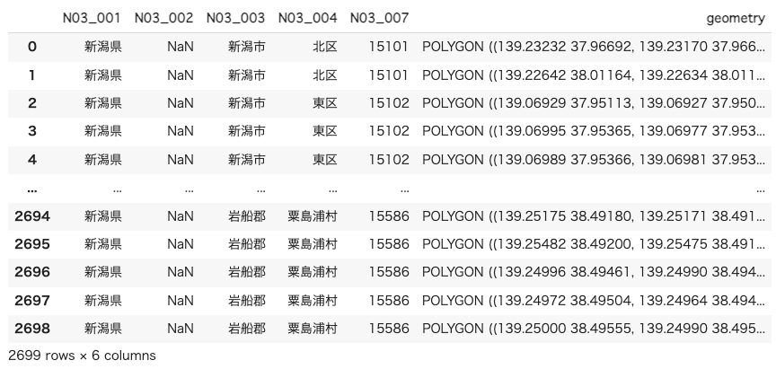
gdf

市区町村ごとのポリゴンデータを取得することができました。

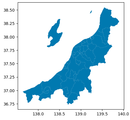
取得したポリゴンデータを表示してみます。

gdf.plot()

上越、中越、下越、岩船、佐渡、魚沼の6地域の市区町村のリストを作成します。
地域区分は新潟県のホームページを参考にしました。

# 市区町村を地域ごとにリスト化
Joetsu = ['上越市' ,'糸魚川市' ,'妙高市']
Tyuetsu = ['加茂市', '三条市', '長岡市','柏崎市', '小千谷市', '十日町市', '見附市', '田上町', '出雲崎町', '刈羽村']
Kaetsu = ['北区', '東区', '中央区', '江南区', '燕市', '秋葉区', '南区',  '西区', '西蒲区', '新発田市', '燕市', '五泉市', '阿賀野市', '胎内市', '聖籠町', '弥彦村', '阿賀町']
Iwafune = ['村上市', '関川村', '粟島浦村']
Sado = ['佐渡市']
Uonuma = ['魚沼市', '南魚沼市', '湯沢町']

Joetsu_gdf = gdf[gdf['N03_004'].isin(Joetsu)]
Tyuetsu_gdf = gdf[gdf['N03_004'].isin(Tyuetsu)]
Kaetsu_gdf = gdf[gdf['N03_004'].isin(Kaetsu)]
Iwafune_gdf = gdf[gdf['N03_004'].isin(Iwafune)]
Sado_gdf = gdf[gdf['N03_004'].isin(Sado)]
Uonuma_gdf = gdf[gdf['N03_004'].isin(Uonuma)]

各地域の月ごとの温度を取得する

GEEの認証を行います。
出力の指示に従って進めてください。

try:
       ee.Initialize()
except Exception as e:
       ee.Authenticate()
       ee.Initialize()

対象地域のポリゴンデータを、GEEで扱うgeometryの属性に変換する関数を定義します。

# 対象地域のポリゴンデータをgeeのgeometryで取得
def get_aoi(gdf_area):
  features = []
  for i in range(len(gdf_area)):
    x,y = gdf_area.iloc[i].geometry.exterior.coords.xy
    coords = np.dstack((x,y)).tolist()
    features.append(coords)
  aoi = ee.Geometry.MultiPolygon(features)
  return aoi

月ごとの平均気温を取得していきます。今回は2022年の1年分のデータを利用します。
地域のループ処理内で月ごとのループ処理を行い、地域ごとの月間気温の推移を取得してリスト(monthly_temp_list)に格納していきます。
LSTの単位はケルビンのため、摂氏への変換も行います。（単純な変換であれば-273.15するだけですが、スケールを加味しないといけないため0.02を掛けています。）

gdf_list = [Joetsu_gdf, Tyuetsu_gdf, Kaetsu_gdf, Iwafune_gdf, Sado_gdf, Uonuma_gdf]

# 月ごとの平均気温を格納するリスト
monthly_temp_list = []

# 地域のループ処理
for gdf in gdf_list:
  # 調査地域のジオメトリを設定
  geometry = get_aoi(gdf)

  monthly_mean_lst = []

  # 対象地域内のMODISデータをフィルタリングする
  start_date = datetime.date(2022, 1, 1)
  end_date = datetime.date(2022, 12, 31)
  n_months = (end_date.year - start_date.year) * 12 + end_date.month - start_date.month + 1

  # 月ごとにループ処理
  for i in range(n_months):
      # 当該月の開始日と終了日を取得
      current_month_start = start_date + relativedelta(months=i)
      current_month_end = min(current_month_start + relativedelta(months=1, days=-1), end_date)

      current_month_start_str = str(current_month_start)
      current_month_end_str = str(current_month_end + datetime.timedelta(days=1))

      try:
          modis_lst = ee.ImageCollection('MODIS/006/MOD11A1').filterDate(current_month_start_str, current_month_end_str).select('LST_Day_1km').filterBounds(geometry)

          # LSTバンドに対して、月ごとの平均値を計算する
          monthly_mean = modis_lst.mean()
          lst_mean = monthly_mean.reduceRegion(reducer=ee.Reducer.mean(), geometry=geometry, scale=1000).get('LST_Day_1km')

          # LST値を摂氏に変換する
          if lst_mean.getInfo() is not None: 
              lst_mean_c = lst_mean.getInfo()*0.02-273.15
              monthly_mean_lst.append((current_month_start.year, current_month_start.month, lst_mean_c))
          else:
              monthly_mean_lst.append((current_month_start.year, current_month_start.month, None))

      except ee.ee_exception.EEException as e:
          print(f"No data available for {current_month_start_str} - {current_month_end_str}: {e}")

  monthly_temp_list.append(monthly_mean_lst)

上で作成した地域ごとのリスト(monthly_temp_list)をグラフで表示します。

x = [f"{year}-{month:02d}" for year, month, _ in monthly_mean_lst]

plt.plot(x, [monthly_mean for _, _, monthly_mean in monthly_temp_list[0]], label='Joetsu')
plt.plot(x, [monthly_mean for _, _, monthly_mean in monthly_temp_list[1]], label='Tyetsu')
plt.plot(x, [monthly_mean for _, _, monthly_mean in monthly_temp_list[2]], label='Kaetsu')
plt.plot(x, [monthly_mean for _, _, monthly_mean in monthly_temp_list[3]], label='Iwafune')
plt.plot(x, [monthly_mean for _, _, monthly_mean in monthly_temp_list[4]], label='Sado')
plt.plot(x, [monthly_mean for _, _, monthly_mean in monthly_temp_list[5]], label='Uonuma')
plt.xlabel('Year-Month')
plt.ylabel('Monthly Mean Temperature (°C)')
plt.title('Monthly Mean Temperature in the Study Area')
plt.xticks(rotation=45)
plt.legend()
plt.show()

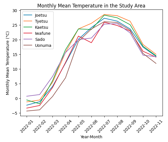
取得できました。
どの地域もだいたい同じような推移をしていることがわかります。(同じ新潟県なので当たり前ですが、、、笑

しかし新潟地方気象台のホームページによると、"年平均気温は山沿いでは11～13℃、海岸・平野部では13～14℃となっています。また、相対的に上越で高く、下越で低くなっています。"とあり、今回の結果とは異なりそうです。この辺はMODISのLSTの特徴や精度をよく調査する必要がありそうです。

まとめ

今回は衛星データのうち、MODISの地表面温度のデータを取得して、新潟県の温度の推移をグラフ化してみました。

宙畑さんで公開している「お米の食味ランク別に農地の様子を衛星データで比較してみたの記事もぜひ読んでいただけると嬉しいです。

今後も衛星データを使って試してみたことを記事にしていきますので、よろしくお願いします。

参考文献

[1]松井 隆，森山雅雄，2008．AIRS データに基づいた MODIS 地表面温度・放射率プロダクトの検証