おおまかな流れ
- NMFとは
- 画像の前処理
- NMFの実装
- 画像の再構成
- 類似度から見込み人気度を予測
- 考察とまとめ
# 今回使用するライブラリなど
import numpy as np
import pandas as pd
from matplotlib import pyplot as plt
from PIL import Image
from typing import Tuple, List, Dict
from sklearn.feature_extraction import image
from sklearn.decomposition import NMF
import pickle
import numbers
from itertools import product
import seaborn as sns
import scipy as sp
%matplotlib inline
1. NMF(非負値行列因子分解)とは
NMF(Nonnegative Matrix Factorization)は機械学習の中でも教師なし学習に分類される手法であり、ざっくりと説明すると複数の画像群などから共通要素(特徴量)を抽出することができます。
数式では以下のように表せます。
X = W・H
X: 元の行列
W: 基底ベクトルの係数行列
H: 任意の数の基底ベクトルが集まった行列
NMFでは名前の通り、X, W, Hの「各行列の要素がすべて非負値」でなければならないという特徴があります。
そのためNMFでは元の行列から得られた任意の数の基底ベクトルに必要な係数をかけたのち、それらの足し合わせのみで元の行列を再構成して表現することができます。
*任意の数の基底ベクトルは行列を表現する際の基盤であり「辞書」とも呼ばれることから、NMFは辞書学習と分類されることがあります。
ゆえに(画像の要素はすべて非負値なので)NMFは画像処理に適した手法であり、またNMFで分解して得られた基底ベクトルを用いて他の画像(行列)を再構成することで異常検知などにも応用可能です。
今回の用途としてはNMFで特定の画像群の特徴量抽出を行い、再構成誤差によってクラスタリングに近いことをします。
具体的には特定の画像群をまとめてNMFで分解することで画像群の傾向を基底ベクトルに反映させ、他の画像群と特定の画像群の間で再構成誤差の数値に差をつけることにより、特定の画像群に属するか否かを判別します。
*NMFに関する詳しい説明は以下のサイトなどを参照してください。
Qiita: 非負値行列因子分解(NMF)をふわっと理解する
あらびき日記: NMF: Non-negative Matrix Factorization(非負値行列因子分解)
2. 画像の前処理
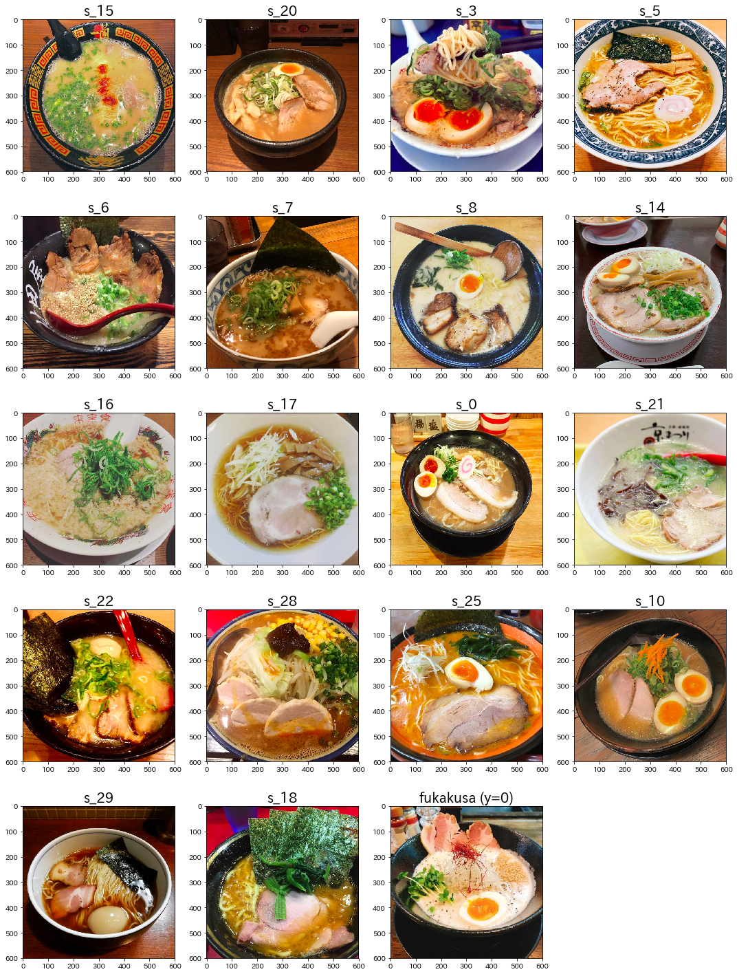
それではNMFで分解させる行列の準備をしていきます。
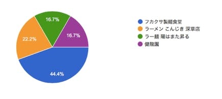
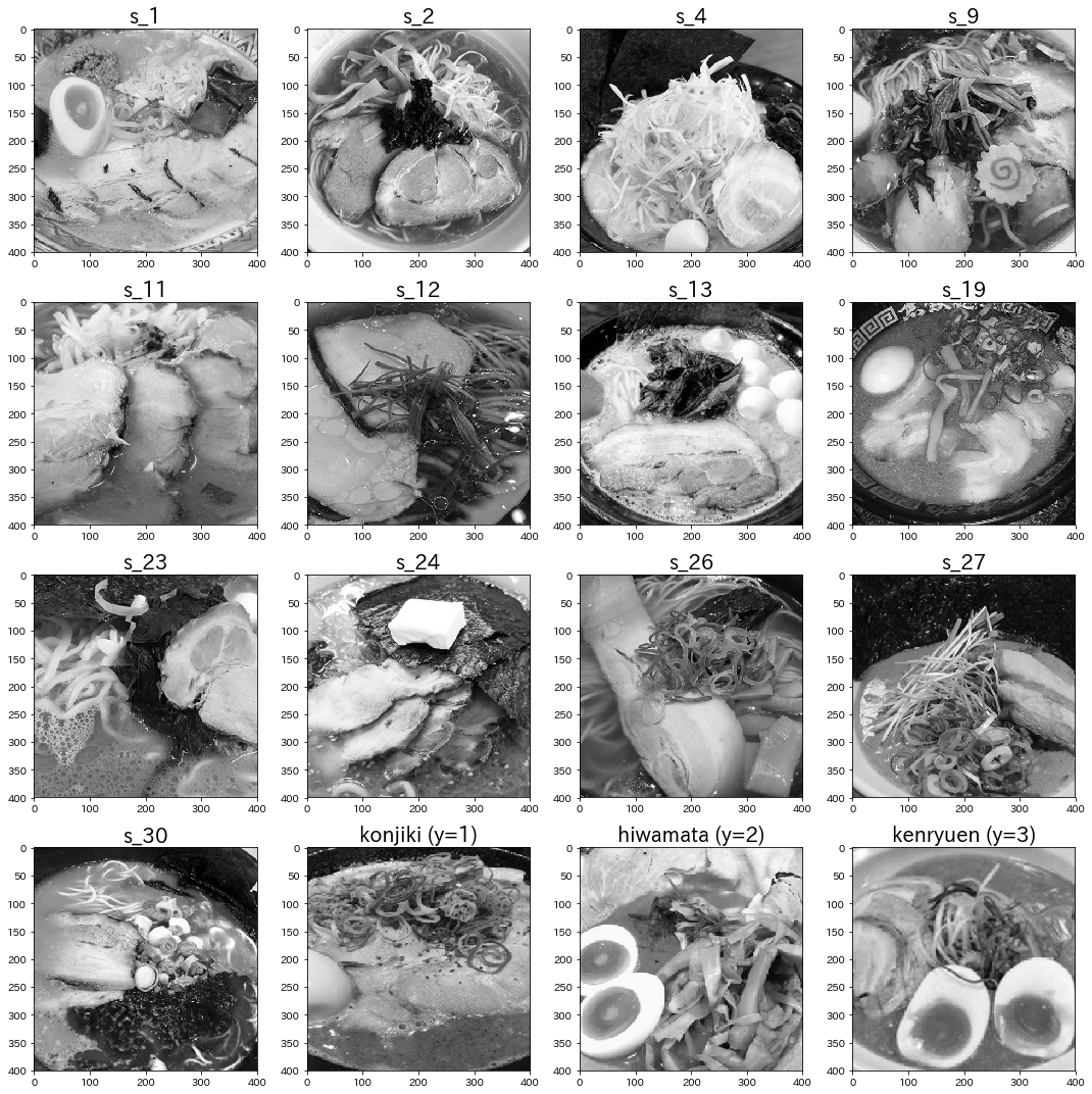
以前の投稿で使用したラーメンの画像群の中から、選ばれる回数が多く事前確率の高かった "フカクサ製麺食堂"(y=0) の画像群を「比較的人気のあるラーメン」と定義し、これらの画像群を元にNMFで特徴量抽出を行い、再構成誤差によってクラスタリングに近いことをします。
要するに、あるラーメン画像をNMFで再構成した際の再構成誤差の数値からこの画像群に属するか否か、つまり「比較的人気のあるラーメン」であるか否かを判断していきます。
ゆえに、その他の画像群は比較対象として精度チェックなどに使用します。
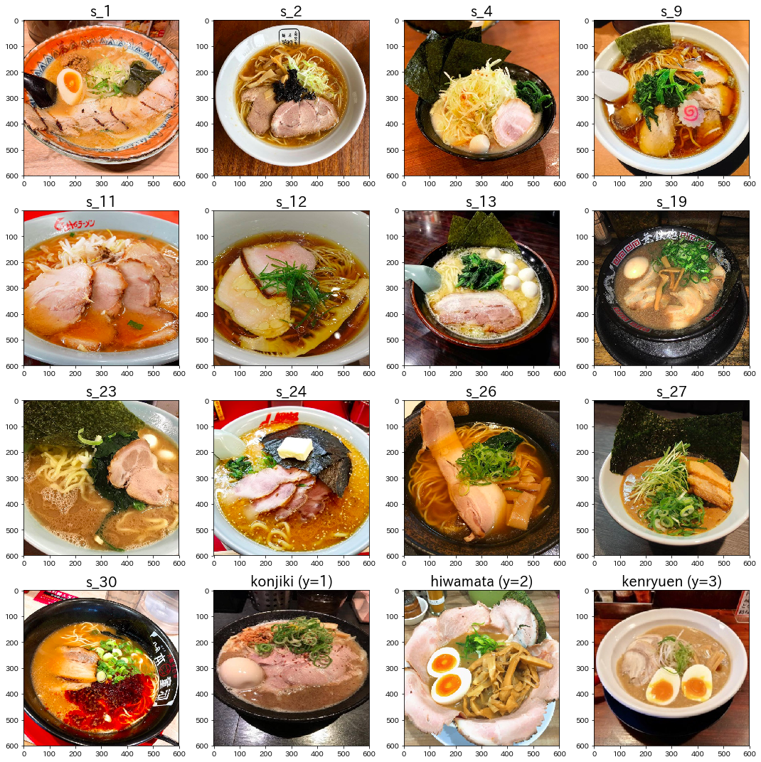
2-1. 画像のトリミング(切り抜き)
まずは各画像で使用する部分のみを(今回は400×400のサイズで)トリミングし、また二次元行列で表現するために色要素を排除してグレースケール化していきます。
*背景やテーブルなどのノイズとなり得る不必要な部分を取り除くことでNMFの精度を向上することができます。
その他の画像群でも同様に処理します。
2-2. 各画像のベクトル化・1つの行列へ集積
更にそれぞれの画像群内の各画像を変形してベクトル化し、それらの各画像ベクトルを集めて1つの行列で表現します。今回はpandasのDataFrameに集積させました。
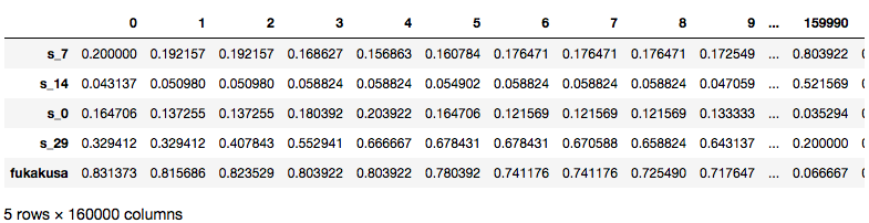
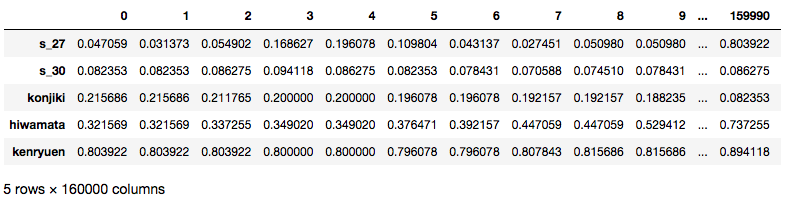
*DataFrameは各行列内のうち5行分のみ表示しています。
2-3. 画像のパッチ(分割)化
次に(ベクトルさせた)各画像を細かく分割してパッチ(小区画の画像)にしていきます。
パッチに分割する理由としては、元のサイズの画像をそのままNMFで基底ベクトルに分解して再構成を試みた場合、表現が複雑なため再構成の精度が落ちてしまうからです。また元のサイズの画像は最初から数に限りがあるため、多くの要素(画像の特徴や枚数)の中からより少ない特徴量(基底ベクトルの数)で元の行列を表現できるというNMFのメリットが薄れてしまいます。
ゆえにパッチに分割することで各パッチ内の表現が単純化され、元のサイズの画像よりも枚数を増加することが可能となり、より精度の高い各パッチの再構成が行われたのち、ジグソーパズルのように元画像の形状へと戻すことで画像全体の再構成精度を向上することができます。
それではまずパッチに分割する関数を用意します。scikit-learn内にパッチ分割ができる関数が既に存在するため、それを元にコードを書いていきます。
def extract_patches(img: np.ndarray, patch_size: Tuple[int, int],
                       extraction_step: int):
    img_height, img_width = img.shape[:2]
    img = img.reshape((img_height, img_width, -1))
    colors = img.shape[-1]
    patch_height, patch_width = patch_size[:2]
    patches = image.extract_patches(img, patch_shape=(patch_height, patch_width, colors),
                                    extraction_step=extraction_step)
    patches = patches.reshape(-1, patch_height, patch_width, colors)
    if patches.shape[-1] == 1:
        return patches.reshape((-1, patch_height, patch_width))
    else:
        return patches
それぞれの画像群内のすべての画像を、今回は20×20のパッチに分割していきます。
*一旦分割したパッチは画像同様、ベクトル化して1つの行列にまとめていきます。
# フカクサ製麺食堂の画像群
patch_list=[]
patches_array=np.ndarray

# imgsにフカクサ製麺食堂の画像群のDataFrameが代入済
for i, row in enumerate(imgs.index):
    img=imgs.loc[row].values.reshape(400, -1)

    # patch making
    patches=extract_patches(img, (20, 20), 20)
    for idx in range(len(patches)):
        patch_list.append(patches[idx].flatten())
patches_array=np.array(patch_list)

print(patches_array.shape)

# その他の画像群
other_patch_list=[]
other_patches_array=np.ndarray

# r_imgsにその他の画像群のDataFrameが代入済
for i, row in enumerate(r_imgs.index):
    img=r_imgs.loc[row].values.reshape(400, -1)

    # patch making
    patches=extract_patches(img, (20, 20), 20)
    for idx in range(len(patches)):
        other_patch_list.append(patches[idx].flatten())
other_patches_array=np.array(other_patch_list)

print(other_patches_array.shape)
出力結果
(7600, 400)
(6400, 400)
これにより要素400(行列にすると20×20)のパッチベクトルが各画像ごとに400枚ずつ取得できました。
念のため、どのようにパッチへ分割されたのか確認してみます。
plt.figure(figsize=(50, 50))
# 1枚の元画像から生成されたパッチをすべて並べる
for i in range(400)):
    plt.subplot(20, 20, i+1)
    plt.imshow(patches_array[7200+i].reshape(20, -1))
出力結果
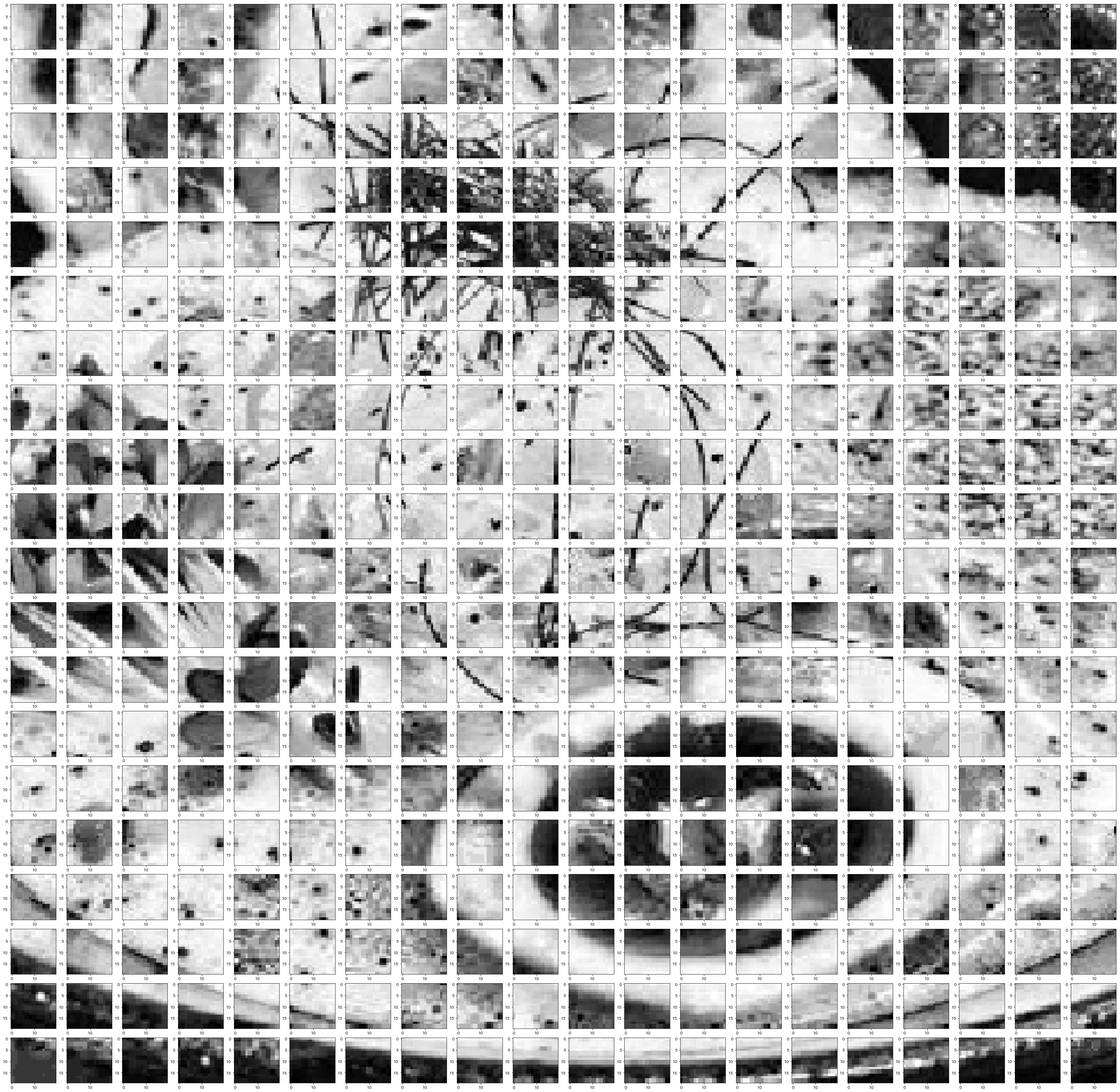
期待通りジグソーパズルのピースように複数のパッチへと分割できました。
3. NMFの実装
必要な前処理がすべて完了したので、早速NMFを実装してみたいと思います。
*NMF自体は、これまたscikit-learnで実装できます。
3-1. パラメータチューニング
NMFの実装にあたって最も考慮すべき点は、基底ベクトルの数を決めるパラメータの"n_components"です。
この"n_components"の値によって再構成の精度が大きく変化するため、とりあえずいくつかの値を用いてNMFを実装しチューニングを行います。
# 複数のmodel格納用のリストを用意
models=[]

# 今回使用するn_componentsの値候補
x=[1, 10, 20, 30, 40, 50, 60, 70, 80, 90, 100]

for n in x:
    model = NMF(n_components=n, init='random', random_state=0)
    # フカクサ製麺食堂の画像群のパッチ行列で学習させる
    model.fit(patches_array)
    models.append(model)
次に学習したNMFモデルがそれぞれどの程度の再構成精度を持つのかを可視化させます。
%%time
# 合計差分とn_componentsの関係を調べる
y=[]
other_y=[]
x=[1, 10, 20, 30, 40, 50, 60, 70, 80, 90, 100]

for n in range(len(x)):

    # フカクサ製麺食堂の画像群のパッチ行列との再構成誤差
    total=0
    error=0

    for i in range(len(patches_array)):
        H=models[n].components_
        W=models[n].transform(patches_array[i].reshape(1, -1))
        X=np.dot(W, H).reshape(20, -1)
        total+=abs(patches_array[i].reshape(20, -1)-X).sum()

    error=total/19
    y.append(error)


    # その他の画像群のパッチ行列との再構成誤差
    other_total=0
    other_error=0

    for i in range(len(other_patches_array)):
        other_H=models[n].components_
        other_W=models[n].transform(other_patches_array[i].reshape(1, -1))
        other_X=np.dot(other_W, other_H).reshape(20, -1)
        other_total+=abs(other_patches_array[i].reshape(20, -1)-other_X).sum()

    other_error=other_total/16
    other_y.append(other_error)

# 結果の可視化
plt.figure(figsize=(10, 10))

# 各再構成誤差の値
plt.subplot(2, 1, 1)
plt.title("NMF reconstruction error values", fontsize=20)
plt.plot(x, y, label="patches")
plt.plot(x, other_y, label="other_patches")
plt.xlabel('n_components', fontsize=15)
plt.ylabel('reconstruction_err_', fontsize=15)
plt.legend()

# 異なる2つの画像群間での再構成誤差の値比較
plt.subplot(2, 1, 2)
plt.title("NMF reconstruction error difference (other_y - y)", fontsize=20)
y_difference=np.array(other_y)-np.array(y)
plt.plot(x, y_difference, label="difference", color="g")
plt.xlabel('n_components', fontsize=15)
plt.ylabel('reconstruction_err_difference', fontsize=15)
plt.legend()

plt.tight_layout()
plt.show()
出力結果 (計算に結構時間がかかります…)
CPU times: user 1h 19min 38s, sys: 16.9 s, total: 1h 19min 55s
Wall time: 53min 15s
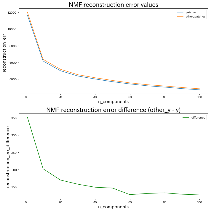
ここから"n_components"の値を選択するにあたり、ポイントとなるのは次の2点です。
1. "n_components"の値を大きくしていくと再構成誤差が小さくなっていく
考えてみれば当たり前ですが、使用できる基底ベクトルが増加すればするほど様々な画像に対応できるようになります。(NMF reconstruction error values内のオレンジと青のグラフ参照)そのため極限まで"n_components"の値を大きくしていけば、再構成誤差は限りなく小さくなります。しかし一方で、その他の画像群のパッチ行列でも同様に再構成誤差が小さくなってしまうため、過度な"n_components"の値の上昇は再構成誤差を小さくしても肝心な「判別の精度」が低下していく可能性が高く、注意が必要です。
2. "n_components"の値を大きくしていくと再構成誤差の値比較に信頼性が増していく
NMF reconstruction error difference (other_y - y)内の緑のグラフの結果から、n_components=1 の時に再構成誤差の値比較が最大となるためこの値を採用できそうにも思われますが、ここでの再構成誤差の値は「複数の画像の平均再構成誤差」であることを忘れてはいけません。**再構成誤差の平均値同士の比較で大きな差が生じたとしても、各画像ごとの再構成誤差の値では"n_components"が小さい分、大きなバラつきが生じている可能性が高く、信頼性が保証できません。**そのため、ある程度"n_components"の値が大きく、再構成誤差の値比較に信頼性があると考えられるグラフ中盤以降の値を採用するのが賢明です。
様々な考え方があると思われますが、私は上記の2点を踏まえて n_components=40 で以降進めていきたいと思います。
3-2. 確定したNMFモデルの辞書画像の表示
それでは採用したパラメータでNMFモデルを実装し、再構成時に使用される辞書画像(行列化させた基底ベクトル群)を表示してみたいと思います。
# モデルの実装
model = NMF(n_components=40, init='random', random_state=0)
model.fit(patches_array)

# 辞書画像の表示
plt.figure(figsize=(15, 10))
for i in range(len(model.components_)):
    plt.subplot(5, 8, i+1)
    plt.imshow(model.components_[i].reshape(20, -1))
出力結果
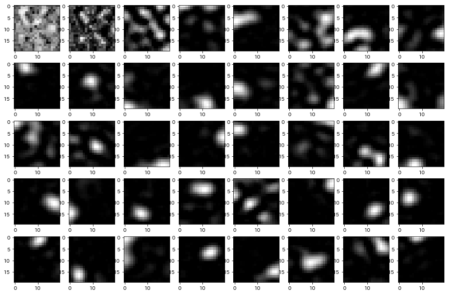
パッチの再構成に使用する辞書画像(行列化させた基底ベクトル群)のため一見意味不明な画像群のようにも見えますが、重みとなる係数が掛け合わせられたこれらの辞書画像を足し合わせることで各パッチを再構成することができます。
(補足) 学習済みNMFモデルの保存・読み込み
必要な時にNMFモデルを毎回学習させるのは骨が折れるため、学習済みNMFモデルを保存しておきます。
# モデルを保存する
filename = 'NMF_model_n40.sav'
pickle.dump(model, open(filename, 'wb'))
"NMF_model_n40.sav" としてファイルが保存されます。
また、保存済みNMFモデルの読み込み方法は以下の通りです。
# 保存したモデルを読み込む
filename = 'NMF_model_n40.sav'
loaded_model = pickle.load(open(filename, 'rb'))
4. 画像の再構成
それでは学習済みのNMFモデルを使用して画像を再構成していきます。
4-1. パッチの再構成
まずはじめに画像内の各パッチを再構成します。
# 1枚の画像からパッチ作成
patch_list=[]
patches_array=np.ndarray

img=imgs.loc["fukakusa"].values.reshape(400, -1)
patches=extract_patches_2d(img, (20, 20), 20)
for idx in range(len(patches)):
        patch_list.append(patches[idx].flatten())
patches_array=np.array(patch_list)


# 各パッチの再構成
total_error=0
transformed_patch_list=[]

plt.figure(figsize=(50, 50))
# reconstructed img
for i in range(len(patches_array)):
    H=loaded_model.components_
    W=loaded_model.transform(patches_array[i].reshape(1, -1))
    X=np.dot(W, H).reshape(20, -1)

    # パッチを1つのリストにまとめていく
    transformed_patch_list.append(X)

    # 再構成誤差の格納
    total_error+=abs(patches_array[i].reshape(20, -1)-X).sum()

    # パッチをすべて並べて表示
    plt.subplot(20, 20, i+1)
    plt.imshow(X)

# パッチをまとめたリストを行列化(次のコードで使用するため)
transformed_patches=np.array(transformed_patch_list)
出力結果
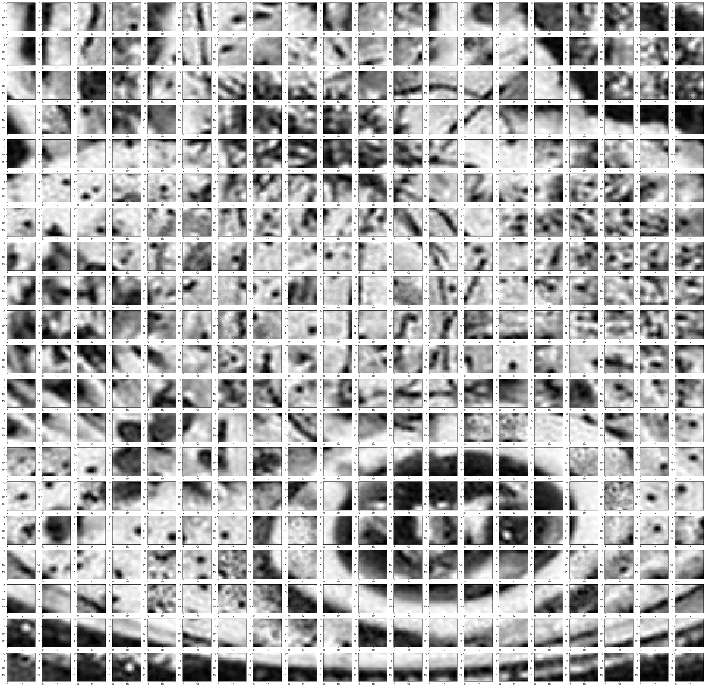
一見意味不明な画像群であった辞書画像(行列化させた基底ベクトル群)から作られたとは思えないほど、それっぽく再構成されていませんか?
4-2. パッチをつなぎ合わせて画像を再構成
それでは分割させてあったパッチを再び元の形につなぎ合わせていきます。
def reconstruct_from_patches(patches: np.ndarray, image_size: Tuple[int, int], extraction_step: int):
    array_ndimension = len(image_size)
    if isinstance(extraction_step, numbers.Number):
        extraction_step = tuple([extraction_step] * array_ndimension)
    img_height, img_width = image_size[:2]
    patch_height, patch_width = patches.shape[1:3]
    extract_height, extract_width = extraction_step[:2]
    img = np.zeros(image_size)
    counter = np.zeros(image_size)
    n_height = (img_height - patch_height) // extract_height + 1
    n_width = (img_width - patch_width) // extract_width + 1
    for p, (i, j) in zip(patches, product(range(n_height), range(n_width))):
        img[extract_height * i:extract_height * i + patch_height, extract_width * j:extract_width * j + patch_width] += p
        counter[extract_height * i:extract_height * i + patch_height, extract_width * j:extract_width * j + patch_width] += 1.
    counter[counter == 0] = 1.
    return img / counter
パッチをつなぎ合わせて画像を再構成する際には、再構成する画像のサイズを指定する必要があります。今回は元画像と同様のサイズである400×400を指定します。
plt.figure(figsize=(10, 5))

# orginal img
plt.subplot(1, 2, 1)
original_img=imgs.loc["fukakusa"].values.reshape(400, -1)
plt.title("fukakusa: original_img", fontsize=20)
plt.imshow(original_img)

# reconstructed img
plt.subplot(1, 2, 2)
reconstructed_img=reconstruct_from_patches(transformed_patches, (400, 400), 20)
plt.title("fukakusa: reconstructed_img", fontsize=20)
plt.imshow(reconstructed_img)

plt.tight_layout()
plt.show()
出力結果
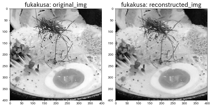
右の画像がNMFによる再構成画像です。結構キレイ。
比較対象として他の画像群でも同様に画像の再構成まで行います。
# 各画像からパッチ作成
names=["konjiki", "hiwamata", "kenryuen"]
img_list=[]

for name in names:
    other_patch_list=[]
    other_patches_array=np.ndarray

    r_img=r_imgs.loc[name].values.reshape(400, -1)
    patches=extract_patches_2d(r_img, (20, 20), 20)
    for idx in range(len(patches)):
            other_patch_list.append(patches[idx].flatten())
    other_patches_array=np.array(other_patch_list)
    img_list.append(other_patches_array)

# 各パッチの再構成
other_total_errors=[]
other_transformed_patches_list=[]

for idx in range(len(img_list)):
    other_total_error=0
    other_transformed_patch_list=[]

    # reconstructed img
    for i in range(len(img_list[idx])):
        H=loaded_model.components_
        W=loaded_model.transform(img_list[idx][i].reshape(1, -1))
        X=np.dot(W, H).reshape(20, -1)

        # パッチを1つのリストにまとめていく
        other_transformed_patch_list.append(X)

        # 再構成誤差の格納
        other_total_error+=abs(img_list[idx][i].reshape(20, -1)-X).sum()

    # パッチをまとめたリストを行列化(次のコードで使用するため)
    other_transformed_patches=np.array(other_transformed_patch_list)


    other_total_errors.append(other_total_error)

    other_transformed_patches_list.append(other_transformed_patches)

# 画像を再構成して表示
plt.figure(figsize=(10, 15))
for i, name in enumerate(names):
    # orginal img
    plt.subplot(3, 2, 1+2*i)
    original_img=r_imgs.loc[name].values.reshape(400, -1)
    plt.title("{}: original_img".format(name), fontsize=20)
    plt.imshow(original_img)

    # reconstructed img
    plt.subplot(3, 2, 2+2*i)
    reconstructed_img=reconstruct_from_patches_2d(other_transformed_patches_list[i], (400, 400), 20)
    plt.title("{}: reconstructed_img".format(name), fontsize=20)
    plt.imshow(reconstructed_img)

plt.tight_layout()
plt.show()
出力結果
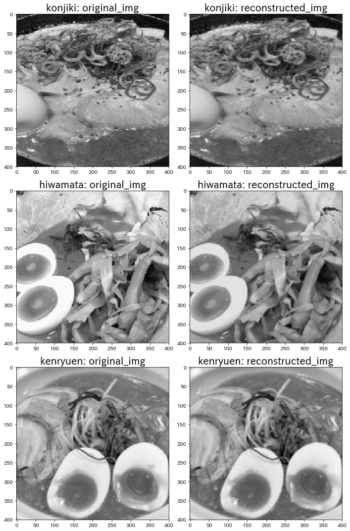
うーん。他の画像でも割と再構成できてる気がします。笑
5. 類似度から見込み人気度を予測
最後に再構成誤差の類似度から見込み人気度を予測していきます。
とりあえず先程再構成した4つの画像の再構成誤差を比較してみます。
*ちなみに再構成誤差は以下のL1ノルム(絶対値誤差)で求めました。
abs(patches_array[i].reshape(20, -1)-X).sum()
イメージとしては画像のまま差分をとって、そこから差分を絶対値に直してから、全体の差分値を足し合わせています。
# n_components=40の時の再構成誤差
print(total_error)
print(other_total_errors)
出力結果
4324.613633481987
[4451.692878038769, 2906.8124369076213, 1503.8777410031942]
結果を見てわかるように、単純な誤差の小ささでは判断できなさそうです。
そのため再構成誤差が正規分布に従うと仮定して、その分布範囲から類似度を判断していきたいと思います。
5-1. 正規分布の形状を予測
とりあえず今ある2つの画像群の再構成誤差データを使用して正規分布を描いてみようと思います。
# もう一度、再構成誤差を「画像ごとに」求めていきます。
totals=[]

for i in range(19):
    total=0

    for idx in range(400):
        H=loaded_model.components_
        W=loaded_model.transform(patches_array[i*400+idx].reshape(1, -1))
        X=np.dot(W, H).reshape(20, -1)
        total+=abs(patches_array[i*400+idx].reshape(20, -1)-X).sum()

    totals.append(total)


other_totals=[]

for i in range(16):
    other_total=0

    for idx in range(400):
        other_H=loaded_model.components_
        other_W=loaded_model.transform(other_patches_array[i*400+idx].reshape(1, -1))
        other_X=np.dot(other_W, other_H).reshape(20, -1)
        other_total+=abs(other_patches_array[i*400+idx].reshape(20, -1)-other_X).sum()

    other_totals.append(other_total)

# 正規分布の表示
plt.figure(figsize=(10, 5))
plt.title("patches gaussian distribution (*actual)", fontsize=20)
sns.distplot(totals, label="patches")
sns.distplot(other_totals, label="other_patches")
plt.legend()
plt.show()
出力結果
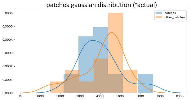
画像が少ない分、イビツな形。しかし、オレンジの正規分布(他の画像群)の方が、青の正規分布(フカクサ製麺食堂の画像群)よりも再構成誤差が若干大きい傾向にあるようです。
それではここから基本統計量をいくつか求めたのち、区間推定をして正規分布の形状を予測していきたいと思います。
*今回は95%の区間推定を行います。
# 不偏分散(ddof=0: 標本分散)
u_var=np.var(totals, ddof=1)
# 平均値
s_mean=np.mean(totals)
# 標準誤差(推定量の標準偏差)
scale=np.sqrt(u_var/len(totals))

# 自由度
deg_of_freedom=len(totals)-1

bottom, up = sp.stats.t.interval(
    alpha=0.95, # 信頼区間
    loc=s_mean,  # 標本平均
    scale=scale, # 標準誤差(推定量の標準偏差)
    df=deg_of_freedom # 自由度
)
print('patchesにおける母平均の95%信頼区間: {:.2f} < μ < {:.2f}'.format(bottom, up))
出力結果
patchesにおける母平均の95%信頼区間: 3491.70 < μ < 4523.34
フカクサ製麺食堂の画像群で95%区間推定ができました。
同様にして、その他の画像群の95%区間推定を行うと以下のようになります。
# 不偏分散(ddof=0: 標本分散)
u_var=np.var(other_totals, ddof=1)
# 平均値
other_s_mean=np.mean(other_totals)
# 標準誤差(推定量の標準偏差)
other_scale=np.sqrt(u_var/len(other_totals))

# 自由度
deg_of_freedom = len(other_totals)-1

bottom, up = sp.stats.t.interval(
    alpha=0.95, # 信頼区間
    loc=other_s_mean,  # 標本平均
    scale=other_scale, # 標準誤差(推定量の標準偏差)
    df=deg_of_freedom # 自由度
)
print('other_patchesにおける母平均の95%信頼区間: {:.2f} < μ < {:.2f}'.format(bottom, up))
出力結果
other_patchesにおける母平均の95%信頼区間: 3560.41 < μ < 4752.69
これらの結果から予測した正規分布の形状を描いてみます。
# 平均と標準偏差から各画像群の正規乱数を1,0000件生成
patches_x = np.random.normal(s_mean, scale, 10000)

other_patches_x = np.random.normal(other_s_mean, other_scale, 10000)


# 予測される正規分布を出力
plt.figure(figsize=(10, 5))
plt.title("patches gaussian distribution (*expected)", fontsize=20)
sns.distplot(patches_x, label="patches")
sns.distplot(other_patches_x, label="other_patches")
plt.legend()

plt.tight_layout()
plt.show()
出力結果
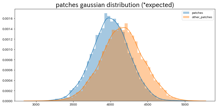
滑らかな正規分布になりました。
また、やはりオレンジの正規分布(他の画像群)の方が、青の正規分布(フカクサ製麺食堂の画像群)よりも再構成誤差が若干大きい傾向にあるという位置関係は正しいようです。
この正規分布のうち青の正規分布(フカクサ製麺食堂の画像群の正規分布)の分布範囲をもとにしてこの画像群との類似度、つまり「ラーメンの見込み人気度」を"割合表記"で最後に予測していきます。
5-2. ラーメンの見込み人気度の割合算出
結論から述べると、以下の関数で求められるようになりました。
def expected_popularity(error_value):

    diff=abs(error_value-4007.523)
    different_rate=diff/(515.818*2)
    if different_rate<=1.0:
        rate=(1.0-different_rate)*100
    else:
        rate=np.random.randint(1, 5)+np.random.rand()

    return round(rate, 1)
この関数に再構成誤差を入れると、まず正規分布の平均値との差が産出されます。そして求めた平均値との差が正規分布の左右どの位置にあるかを正規分布の中央からのズレ具合で割合を数値化します。
また求めた平均値との差が正規分布の範囲から確実に外れてしまっている画像に対しては、正規分布95%の範囲には含まれないからと言って、残り5%の両端部分にも含まれていない可能性を完全に無視することはできないとして、ランダムで1.0% ~ 4.9%の確率が付与されます。
よって、ラーメンの見込み人気度は以下のように算出されます。
print("Expected Popularity (the higher, the better)")
print("fukakusa: "+str(expected_popularity(total_error))+"%")

print("\n")

print("Expected Popularity (the lower, the better)")
names=["konjiki", "hiwamata", "kenryuen"]
for i in range(len(other_total_errors)):
    print(names[i]+": "+str(expected_popularity(other_total_errors[i]))+"%")
出力結果
Expected Popularity (the higher, the better)
fukakusa: 69.3%
Expected Popularity (the lower, the better)
konjiki: 56.9%
hiwamata: 3.3%
kenryuen: 3.4%
期待していた通り、フカクサ製麺食堂のラーメンの見込み人気度が比較的高く、逆にその他の画像群のラーメンの見込み人気度は比較的低めに算出されました。
*結果はあくまで私の大学ゼミ内の意見のみを反映させたものです。
6. 考察とまとめ
今回のNMFによる特徴量抽出では、7600枚のパッチから僅か40枚程度の辞書画像で元画像をかなり忠実に再構成できるという結果に終わりました。
これはNMFの汎用性と可能性を示す良い一例と言えるでしょう。
今後について
前回同様、今回の人気度予測システムもflaskにてwebアプリ化していきたい。
開発環境
jupyter Notebook 5.7.4
参考URL
Qiita: 非負値行列因子分解(NMF)をふわっと理解する
あらびき日記: NMF: Non-negative Matrix Factorization(非負値行列因子分解)
統計WEB: 統計学の時間