続き・・・
以下前回の記事
Twitterのいいね数を推定してみる
ツイートの内容からいいね数を推定するというものです。
今回は精度を求めていきます。
データセットの見直し
データがあまりにも少なすぎるのでもっと関係がありそうな項目を取得していきます。
とは言ってもそんなに伸びツイートか否かに使えそうだなぁと思えたのは以下の2つでした。
- リプライか否か
- 引用リツイートか否か
この2つを追加してみます。
    # ユーザーを指定して取得 (screen_name)
    getter = TweetsGetter.byUser('hana_oba')
    df = pd.DataFrame(columns = ['week_day','have_photo','have_video','tweet_time','text_len','favorite_count','retweet_count','quoted_status','reply','year_2018','year_2019','year_2020'])

    cnt = 0
    for tweet in getter.collect(total = 10000):
        cnt += 1

        week_day = tweet['created_at'].split()[0]
        tweet_time = tweet['created_at'].split()[3][:2]
        year = tweet['created_at'].split()[5]

        # Eoncodeしたい列をリストで指定。もちろん複数指定可能。
        list_cols = ['week_day']
        # OneHotEncodeしたい列を指定。Nullや不明の場合の補完方法も指定。
        ce_ohe = ce.OneHotEncoder(cols=list_cols,handle_unknown='impute')

        photo = 0
        video = 0
        quoted_status = 0
        reply = 0
        yar_2018 = 0
        yar_2019 = 0
        yar_2020 = 0

        if 'media' in tweet['entities']:

            if 'photo' in tweet['entities']['media'][0]['expanded_url']:
                photo = 1
            else:
                video = 1

        if 'quoted_status_id' in tweet:
            quoted_status = 1
        else:
            quoted_status = 0

        if tweet['in_reply_to_user_id_str'] is None:
            reply = 0
        else:
            reply = 1
        if year == '2018':
            yar_2018 = 1
            yar_2019 = 0
            yar_2020 = 0
        if year == '2019':
            yar_2018 = 0
            yar_2019 = 1
            yar_2020 = 0
        if year == '2020':
            yar_2018 = 0
            yar_2019 = 0
            yar_2020 = 1


        df = df.append(pd.Series([week_day, photo, video, int(tweet_time), len(tweet['text']),tweet['favorite_count'],tweet['retweet_count'],quoted_status,reply,yar_2018,yar_2019,yar_2020], index=df.columns),ignore_index=True)
        df_session_ce_onehot = ce_ohe.fit_transform(df)

    df_session_ce_onehot.to_csv('oba_hana_data.csv',index=False)
これでスコアを出してみます。
datapath = '/content/drive/My Drive/data_science/'
df = pd.read_csv(datapath + 'oba_hana_data.csv')

train_count = int(df.shape[0]*0.7)
df_train = df.sample(n=train_count)
df_test = df.drop(df_train.index)

have_photo = 'have_photo'
have_video = 'have_video'
tweet_time = 'tweet_time'
text_len = 'text_len'
favorite_count = 'favorite_count'
retweet_count = 'retweet_count'
quoted_status = 'quoted_status'
reply = 'reply'
year_2018 = 'year_2018'
year_2019 = 'year_2019'
year_2020 = 'year_2020'


# モデルの宣言
from sklearn.ensemble import RandomForestRegressor

# 外れ値除去
df_train = df_train[df_train['favorite_count'] < 4500]
df_train.shape

x_train = df_train.loc[:,[have_photo,have_video,tweet_time,text_len,quoted_status,reply,year_2018,year_2019,year_2020]]
t_train = df_train['favorite_count']
x_test = df_test.loc[:,[have_photo,have_video,tweet_time,text_len,quoted_status,reply,year_2018,year_2019,year_2020]]
t_test = df_test['favorite_count']

# モデルの宣言
model = RandomForestRegressor(n_estimators=2000, max_depth=10,
                                min_samples_leaf=4, max_features=0.2, random_state=0)

# モデルの学習
model.fit(x_train, t_train)
# モデルの検証
print(model.score(x_train, t_train))
print(model.score(x_test, t_test))
0.7189988420451674
0.6471214647821018

飛躍的に精度が上昇しました!
引用リツイートか否かはそこまで寄与度は高くありませんが曜日ほど無関係ではなさそうです。
ただ、もう一つ気になっていたのがツイート時間。現在ただの数値として見ていますのでいくつかの帯域に分けてみた方がよさそうです。
time_mean = pd.DataFrame(columns = ['time','favorite_mean'])
time_array = range(23)
for i in range(23):
  time_mean = time_mean.append(pd.Series([i,df_train[df_train['tweet_time'] == time_array[i]].favorite_count.mean()], index=time_mean.columns),ignore_index=True)

time_mean['time'] = time_mean['time'].astype(int)

sns.set_style('darkgrid')
plt.figure(figsize=(12, 8))
sns.catplot(x="time", y="favorite_mean", data=time_mean,
                height=6, kind="bar", palette="muted")
plt.show()

※時間は標準時です
イコラブのメンバーはSNSは24時までと決まりがあるので(少しはみ出てもセーフ)0の部分もありますがそれ以外だと日本時間の24時台(おそらくお誕生日おめでとうなツイート)は平均値が高いことがわかります。
↑ではいくつかの帯域別に分けた方がいいといいましたがおそらくこれは帯域に分けるのではなくTargetEncodingの方がいいでしょう(ざっくりと時間で分けるのが難しそうなため)
pip install category_encoders

from category_encoders.target_encoder import TargetEncoder
df_train["tweet_time"] = df_train["tweet_time"].astype(str)

TE = TargetEncoder(smoothing=0.1)

df_train["target_enc_tweet_time"] = TE.fit_transform(df_train["tweet_time"],df_train["favorite_count"])
df_test["target_enc_tweet_time"] = TE.transform(df_test["tweet_time"])
tweet_timeの代わりにtarget_enc_tweet_timeを用いて学習し、そのスコアを見てみます
0.6999237089367164
0.6574824327192588
訓練データの方は下がりましたが検証データの方は上がりました。
ちなみにtweet_time、target_enc_tweet_timeの両者を採用すると以下のようになりました。
0.7210047209796951
0.6457969793382683
訓練データでのスコアは一番良いですが検証データでは一番よくありません。
どれも甲乙つけがたいですが一旦どの可能性も残しておいて次に行きましょう。
モデルの変更
今はランダムフォレストで設定も何もいじっていません。そこでモデルをXGBoostにし、optuna を使って最適なパラメータを見つけていきたいと思います。
optunaをインストールします
!pip install optuna
続いてXGboostをoptunaで回せるように関数化していきます。
ここで、それぞれのハイパーパラメータの値に適当な数値が並んでいますがこれは何回も繰り返していくうえで微調整していきます。
# XGboostのライブラリをインポート
import xgboost as xgb
# モデルのインスタンス作成
# mod = xgb.XGBRegressor()
import optuna

def objective(trial):
    # ハイパーパラメータの候補設定
    min_child_samples = trial.suggest_int('min_child_samples', 60, 75)
    max_depth  = trial.suggest_int('max_depth', -60, -40)
    learning_rate   = trial.suggest_uniform('suggest_uniform ', 0.075, 0.076)
    min_child_weight = trial.suggest_uniform('min_child_weight', 0.1, 0.8)
    num_leaves = trial.suggest_int('num_leaves', 2, 3)
    n_estimators = trial.suggest_int('n_estimators', 100, 180)
    subsample_for_bin = trial.suggest_int('subsample_for_bin', 450000, 600000)

    model = xgb.XGBRegressor(min_child_samples = min_child_samples,min_child_weight = min_child_weight,
                          num_leaves = num_leaves,subsample_for_bin = subsample_for_bin,learning_rate = learning_rate,
                          n_estimators = n_estimators)


    # 学習
    model.fit(x_train, t_train)

    # 評価を返す
    return (1 - model.score(x_test, t_test))
まずは100回回してみましょう。
# 試行回数を指定
study = optuna.create_study()
study.optimize(objective, n_trials=100)

print('ハイパーパラメータ:', study.best_params)
print('精度:', 1 - study.best_value)
それぞれでスコアを見てみます
①tweet_timeのみ採用
0.690093409305073
0.663908038217022
②target_enc_tweet_time のみ採用
0.6966901697205284
0.667797061960107
③tweet_timeとtarget_enc_tweet_time 両採用
0.6972461315076879
0.6669948080176482
わずかではありますが②が一番精度が良いようです。
ありとあらゆる可能性を試した方がいいに決まっているのですが、もしここから1つに絞るならばどれが一番よいのでしょうか?
②と③はほとんど変わりませんが②が検証データでスコアが良く、③は訓練でスコアが良い。
ここからoptunaで精度を高めるべく微調整をする場合
- 訓練のスコアが高い方が伸びしろが高いと取るか
- 検証のスコアが高い方が過学習がひどくないのでもっと精度を上げていく
のどちらを考えるべきなんでしょう?
どちらかと言い切れる問題ではないかもしれませんが一般的にどちらが正しい道筋なのか知ってる方いらしたら教えていただけると幸いです。
今回は②を極める方で進めていきます。
ハイパーパラメータの範囲を一旦広く持ち、試行回数を1000回に増やします。
それで得られた最良の結果のときのハイパーパラメータ付近に範囲を狭め、再度1000回試行。
これで得られた結果が以下です。
0.6962221939011508
0.6685252235753019
これまでで一番よい検証結果が得られました。
僕が知っている精度向上の方法はすべて試したので今回はここまでにします。
最後に推論結果と実際の値のヒストグラムを見てみましょう。

本当は1600当たりにある山が何に引っ張られて作られているのかがわかればよかったですね。
最初に出した精度の低い時と何が変わったか、パッとわからないあたりプロットするグラフの種類を間違えたかな…
見にくいですがオレンジ:本当のいいね数、緑:推論したいいね数、青:誤差
でプロットしてみました。
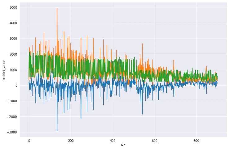
基本的に低めに推論していますね。やはり大場花菜はAIの予測を上回るツイートをしているわけか・・・(お前のモデルをはAI呼べる代物じゃない)
Fin