とある弊社のデータセットで回帰予測

はじめに

はじめましてnyanko-boxです。これまでのQiita歴はたまにコメントする程度でROM専に近い状況でしたが、業務で行っている回帰予測がそこそこ動き出したので初投稿しようと思います。機械学習/深層学習を学び始めて1年強 (2019/03/25現在) でまだまだ拙いところは多いですが、「これを読む後輩がプロジェクトの状況を理解できますように」「Qiitaの諸先輩方からマサカリを貰ってスキルアップしよう」などという期待が込められています。

TL;DR

• LSTM2層+全結合1層でネットワークを構築
• とある弊社のデータセットで回帰予測を実施
• 後出し予測死...?

環境

• Windows10 pro (+GTX1080ti)
• Python3.6.7 (Anaconda)
• TensorFlow1.13

使用するデータ

• 1分毎にロギングされたセンサデータ
  • 日付を適当なものに振り直し済み
  • 平均0, 分散1の系列に変換済み

import pandas as pd
dataset = pd.read_csv(filepath, parse_dates=["Date"], index_col=["Date"], dtype="float32")
dataset.info()
print("target_0 mean: %f, std: %f" % (dataset["target_0"].std(), dataset["target_0"].mean()))

<class 'pandas.core.frame.DataFrame'>
DatetimeIndex: 236185 entries, 2018-01-01 00:00:00 to 2018-06-14 00:24:00
Data columns (total 26 columns):
target_0    236185 non-null float32
target_1    236185 non-null float32
target_2    236185 non-null float32
target_3    236185 non-null float32
input_0     236185 non-null float32
input_1     236185 non-null float32
input_2     236185 non-null float32
input_3     236185 non-null float32
input_4     236185 non-null float32
input_5     236185 non-null float32
input_6     236185 non-null float32
input_7     236185 non-null float32
input_8     236185 non-null float32
input_9     236185 non-null float32
input_10    236185 non-null float32
input_11    236185 non-null float32
input_12    236185 non-null float32
input_13    236185 non-null float32
input_14    236185 non-null float32
input_15    236185 non-null float32
input_16    236185 non-null float32
input_17    236185 non-null float32
input_18    236185 non-null float32
input_19    236185 non-null float32
input_20    236185 non-null float32
input_21    236185 non-null float32
dtypes: float32(26)
memory usage: 25.2 MB
target_0 mean: 1.000021, std: -0.000112

処理内容

前処理

差分系列変換

今回モデル学習にあたって、センサのログデータを下記のように整形しています。

• datasetの前8割を学習/検証用、残り2割を予測用として使用
• モデルへの入力: 現在の値$-$過去の値
• モデル出力に対する教師: 未来の値$-$現在の値

l_learn = int(dataset.shape[0]*0.8)
training_set = dataset.iloc[:l_learn, :]
predict_set  = dataset.iloc[l_learn:, :]

# 入力
diff_training_set = training_set - training_set.shift(l_diff)
diff_predict_set = predict_set - predict_set.shift(l_diff)

# 出力
tgt_cols = ["target_0", "target_1", "target_2", "target_3"]
target_training_set = training_set[tgt_cols].shift(-l_pred) - training_set[tgt_cols]
target_predict_set  = predict_set[tgt_cols].shift(-l_pred) - predict_set[tgt_cols]

デルタパラメータ

後述するセンサデータの差分のほか、学習には各系列のデルタパラメータを用います。ここでデルタパラメータとは、フォーカスしている時刻からnステップ遡ったサンプル点たちを用いて線形回帰を行い、その係数をもって系列が増加傾向・停滞・減少傾向のいずれかの状態にあることを示す特徴量としています。デルタパラメータの算出に際してnの値は、目的変数 (target_0~3) の変化に対して、説明変数 (input_0~21) における前兆がどれくらい前から発生するかを事前に調べて設定しています。また前項で差分系列の話をしていますが、デルタパラメータの計算には原系列を用いています。

import numpy as np
from sklearn.linear_model import LinearRegression
from numba import jit, u2, f4

@jit(f4[:,:](f4[:,:], u2, u2[:]))
def calc_deltap_core(arg_arr, n, x): # xは回帰係数計算用のダミーarray
    l = arg_arr.shape[0]
    w = arg_arr.shape[1]
    d_params = []
    for ts_line in arg_arr.T:
        # 入力変数1つずつ処理
        temp_lis = []
        for i in range(n, l):
            # 1本の時系列データに関してn個ずつ処理
            param = ts_line[i-n:i]
            regmodel = LinearRegression(normalize=True)
            regmodel.fit(x.reshape(-1, 1), param)
            temp_lis.append(regmodel.coef_.tolist())

        d_params.append(temp_lis)

    d_params_arr = np.array(d_params)
    d_params = d_params_arr.reshape(d_params_arr.shape[0], d_params_arr.shape[1])

    return d_params.T

deltas_training0 = calc_deltap_core(training_set, n, hax)

結合

前々項、前項で計算した差分系列とデルタパラメータを結合して入力データセットとします。
また差分処理やデルタパラメータの算出時にデータセットのheadとtailにnanが存在しますので、結合後にまとめて除去します。

# 結合 (デルタパラメータは2種類のnを用いて計算しているため0と1がある)
input_training_set = pd.concat((diff_training_set, deltas_training0, deltas_training1), axis=1)
input_predict_set = pd.concat((diff_predict_set, deltas_predict0, deltas_predict1), axis=1)

# nan除去
input_training_set = input_training_set.iloc[num_head_nan:-num_tail_nan,:]
target_training_set = target_training_set.iloc[num_head_nan:-num_tail_nan,:]
input_predict_set = input_predict_set.iloc[num_head_nan:-num_tail_nan,:]
target_predict_set = target_predict_set.iloc[num_head_nan:-num_tail_nan,:]

モデル学習

モデル生成

学習モデルを構成していきます。今回はLSTMを2層、全結合層を1層設けています。LSTMなのでlength_of_sequenceを調整すれば活躍してくれそうな気配を感じるところですが、いろいろ変えて計算を回してみたところ学習がうまくできていませんでした。1ステップ毎に計算した結果が現状最も良い結果を見せているので、ここではlength_of_sequence=1としています。

from tensorflow.keras import backend as K
from tensorflow.keras import regularizers
from tensorflow.keras.models import Sequential
from tensorflow.keras.layers import Dense, Activation, CuDNNLSTM, Dropout
from tensorflow.keras.optimizers import SGD

def fit_cudnnlstm(a_verbose, 
                  exps, targets, 
                  a_lr, 
                  a_unit_lstm1, a_unit_lstm2, 
                  a_epoch, a_batch, 
                  a_unit_ff1=None, a_penalty=None, a_do_r=None):
    K.clear_session()

    input_exp = exps.reshape((exps.shape[0], 1, exps.shape[1])) # length_of_sequence=1

    # モデル定義
    model = Sequential()
    model.add(CuDNNLSTM(a_unit_lstm1, return_sequences=True,
                        input_shape=(input_exp.shape[1], input_exp.shape[2])))
    model.add(CuDNNLSTM(a_unit_lstm2, return_sequences=False))

    if a_unit_ff1 != None:
        if a_penalty != None:
            model.add(Dense(a_unit_ff1, kernel_regularizer=regularizers.l2(a_penalty)))
        else:
            model.add(Dense(a_unit_ff1))
        if a_do_r != None:
            model.add(Dropout(a_do_r))
        model.add(Activation("tanh"))

    model.add(Dense(targets.shape[1]))
    model.add(Activation("tanh"))

    model.compile(loss="mean_absolute_error", optimizer=SGD(lr=a_lr))

    history = model.fit(input_exp, targets,
                        epochs=a_epoch,
                        batch_size=a_batch,
                        verbose=a_verbose,
                        shuffle=False,
                        validation_split=0.3
                       )

    return model, history

パラメータ探索

Optunaを使用してユニット数を探索しています。regularizers.l2の値も探索できるようにしていますが、一先ず正則化無しでユニット数のみを対象に探索した結果を投稿します。
Optunaのtimeoutで探索を時間指定できるのが便利ですね。夕方回して次の日の朝に結果を見るとか

import optuna

def optimize_objective(trial):
    # --- 探索するパラメータの設定 ---------------------------------------------------------
    param_unit_lstm1  = int(trial.suggest_discrete_uniform("num_unit_lstm1", 8, 512, 16))
    param_unit_lstm2  = int(trial.suggest_discrete_uniform("num_unit_lstm2", 8, 512, 16))
    param_unit_ff1  = int(trial.suggest_discrete_uniform("num_unit_ff1", 8, 512, 16))
    param_lr  = 0.001
    # --- 静的なパラメータ ----------------------------------------------------------------
    n_epoch = 200
    n_batch = 64
    #-------------------------------------------------------------------------------------

    # データ数をbatch_sizeの倍数にするため時系列的に古いデータを切り捨て
    input_arr = input_training_set[input_training_set.shape[0]%n_batch:, :]
    target_arr = target_training_set[target_training_set.shape[0]%n_batch:, :]

    # モデルフィット
    opt_model, opt_history = fit_cudnnlstm(0,
                                           input_arr, target_arr,
                                           param_lr,
                                           param_unit_lstm1, 
                                           param_unit_lstm2, 
                                           n_epoch, n_batch,
                                           param_unit_ff1)

    # 評価
    return opt_history.history["val_loss"][-1]

limit_sec = 60*60*(24*2+14) # [sec.] 金曜の夕方に探索を開始して月曜の朝に結果が見られるような調整
study = optuna.create_study()
study.optimize(optimize_objective, timeout=limit_sec)

結果

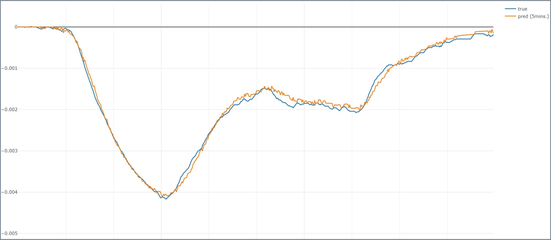
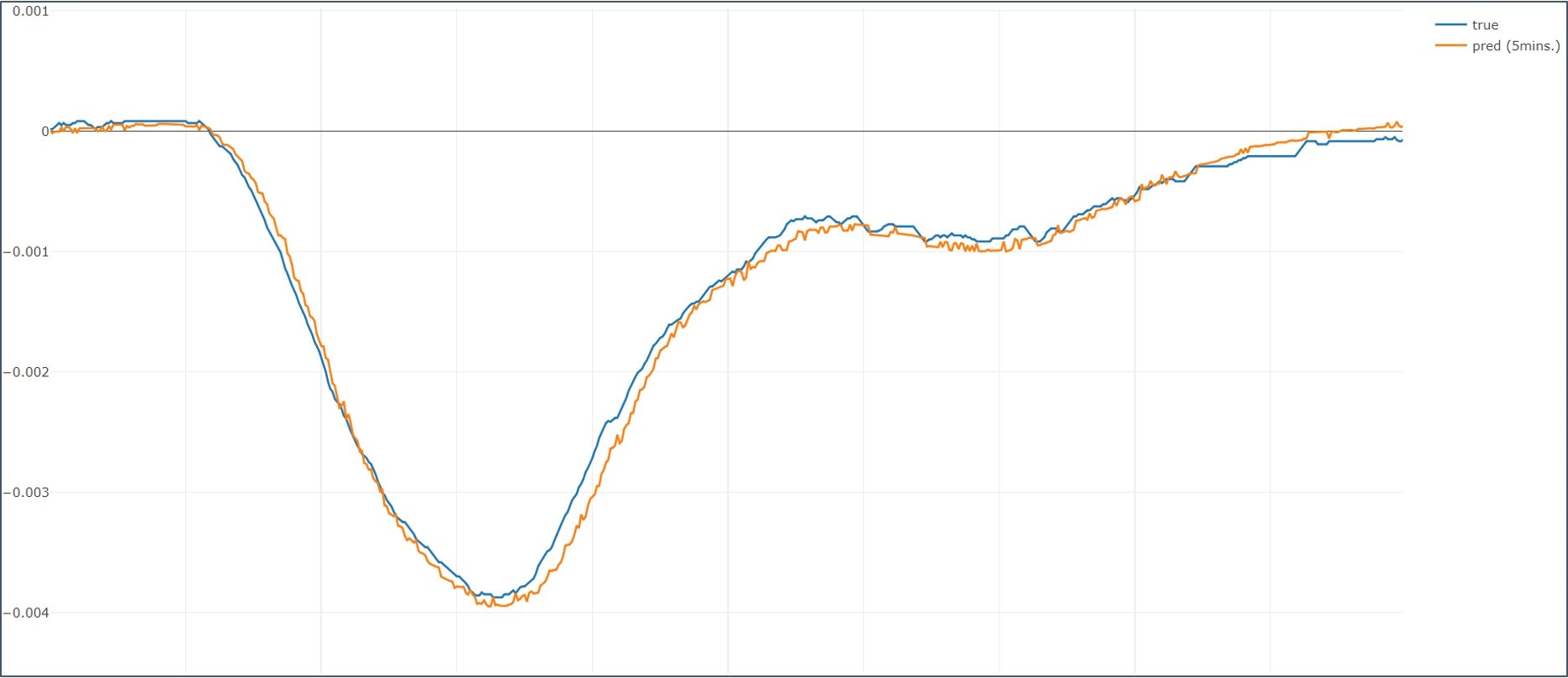
探索の結果、{'num_unit_lstm1': 96.0, 'num_unit_lstm2': 176.0, 'num_unit_ff1': 256.0}という条件で最もval_lossが小さくなりました。この条件で予測用データセットを入力し、得られた予測値と正解の比較を下図に示します。意図的に縦軸と横軸を消してありますがお察しください。

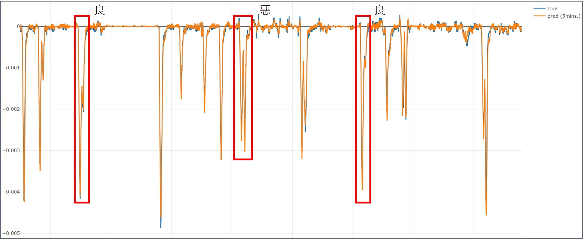
点数が点数なので引きで見ると良い結果が出ていますが、機械学習界隈でおなじみの "良すぎる結果は信じるな" 状態です。
赤枠たちをそれぞれ拡大したものを列挙していきます。

• 良1 (左側)
  

• 良2 (右側)
  

• 悪
  

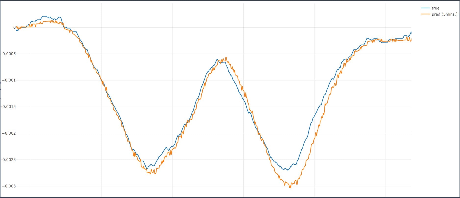
悪い結果を見ると、多峰性となっている変化の鞍部分で予測が後追いになっています。良結果の方では、甘め評価で見て「まぁこれなら後追いじゃあない...かな?」くらいの結果になっていますのでこれだと使う側が活用できないなぁという状況です。
良結果も出てはいるので、この結果を踏まえて社内業務に仮デプロイする予定です。

まとめ

• Qiita ROM専だった私が初投稿してみました。
• LSTM2層と全結合1層で回帰予測を行いました。
• 良い結果ばかりではないですが、社内業務への仮デプロイとしては期待を持っても良いのではないでしょうか
• マサカリいただけるととても喜びます