■0.はじめに
以下の資格を取得しました。
本記事は、資格取得の過程で得た自身の知識の整理、定着化を狙って作成したものです。
今後、資格取得を目指している方のお役に立てれば幸いです。
なお、章立ては主教材に沿っていますが、試験勉強始めた時点で知っていた個所などは内容が薄くなっております。
ご了承ください。
★試験内容★
- 概要:Pythonを使ったデータ分析の基礎や方法を問う試験
- 問題数:40問(すべて選択問題)
- 合格ライン:正答率70%
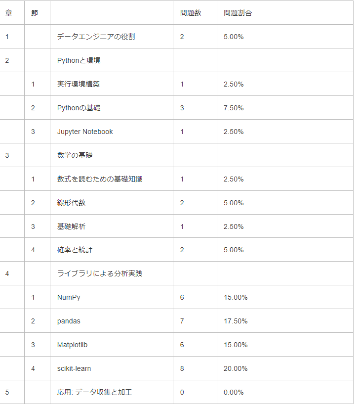
- 出題範囲:主教材である翔泳社「Pythonによるあたらしいデータ分析の教科書」より以下の範囲と割合で出題
★私が行った試験対策★
▼受験前のスペック
- 仕事では下記で記事にした業務改善で少し使用した程度
- プライベートでの使用歴は5年程度
- データ分析・可視化での利用がほとんどで、pandas、Matplotlibはそれなりに使える
- scikit-learnはあまり詳しくない
▼勉強方法
・主教材を読み込む
- 出題範囲である4章までを3回ほど通して読み込みました
- 本に記載されていない内容も一部出題されていましたが、ほとんどは記載されている内容からの出題なので、主教材を読み込むというのが効率的な学習方法だと私は感じました
- 主教材を読み込んで理解が浅いと感じた個所は、サンプルコードを実際に書いて動かして理解を深めました
- 理解した内容を整理してまとめる(本記事)
・公式サイトで紹介されていた模擬試験を繰り返し解き、間違った個所や理解が浅いと感じた個所を学び直す
-
プライム・ストラテジー
- ユーザー登録不要
- 試験開始時に入力するメールアドレスに試験結果が通知される
- 試験問題は3パターン固定
- 内1つは解説付きだが、残り2つは正誤のみで解説なし
-
DIVE INTO CODE
- ユーザー登録が必要
- 問題はランダムで出題
- 課金することで出題範囲を絞り込むことが可能なよう(私はやってません)
出題形式は後者の方が実際の試験に近く、試験の方が若干難しかったように感じました。
メソッドのデフォルト値を理解できているかを確認するような設問など、想定していたより細かい知識を問われる問題も見られ、ある程度実際にコードを書いて動作を理解しておく必要があると感じました。
■1.データエンジニアの役割
データ分析の世界
- データ分析の分野において、プログラミング言語Pythonはデファクトスタンダードな存在になっている
- Pythonの特徴
- 言語としての仕様がわかりやすい
- コンパイル不要な動的スクリプト言語
- 豊富な標準ライブラリと外部のパッケージ
- データ分析以外にも応用範囲が広い
- オープンソース
- Pythonが得意とする分野
- サーバー系ツール
- Webシステムの構築
- IoTデバイスの操作
- 3Dグラフィックス
- Pythonが苦手とする分野
- Webアプリなどのフロントエンド
- デスクトップGUI
- 速度向上などのための低レイヤー処理
- 超大規模かつミッションクリティカルな処理
- Python以外の選択肢
- R言語
- RにはC++を使うためのパッケージが存在し、高速化をする際によく用いられる
- Excel
- R言語
- データサイエンティストとは
- データ分析またはデータ解析の一連の処理及び理解・評価を行える立場の職種
- 研究分野と実務で役割に多少の違いがある
- 研究分野:新たな解法、新技術への取り組みが重視される
- 実務:解決したい課題に向き合うことが重視される
- データ分析エンジニアとは
- データベース技術からデータの活用までデータに関わる幅広い分野に広がっているデータ工学を実践する1つの職種として位置づけられる
- 持つべき技術
- データの入手や加工などのハンドリング
- データの可視化
- プログラミング
- インフラレイヤー
- データハンドリング(前処理)の重要性
- データ分析を行う上で非常に重要な役割を持つ
- 機械学習において業務の8割とも9割とも言われている
- データの入手や再加工、つなぎ合わせや可視化など、分析を行う上で何度も繰り返し実行する
機械学習の位置づけと流れ
- 機械学習とは
- 機械学習で予測を行うためのモデルを作り、データのカテゴライズや数値予測を行っていく
- 機械学習以外の選択肢
- ルールベース:条件分岐の要領で、if分の条件を書いていくというアプローチ
- 統計的な手法:データから統計的な数値を求め、それらの数値に沿うように予測するアプローチ
- 機械学習のタスク
- 教師あり学習
- 正解となるラベルデータが存在する場合に用いられる方式
- 目的変数:正解ラベルである目的データ
- 説明変数(特徴データ、特徴量):目的変数を説明するためのデータ
- 目的変数の種類により回帰と分類の2種類に分けられる
- 回帰:目的変数が連続値になる
- 分類:目的変数がカテゴライズされているデータとなる
- 教師なし学習
- 正解ラベルを用いない学習方法で、主にクラスタリングや次元削減といったタスクを行う
- クラスタリング:与えられたデータの中からグルーピングを行っていく
- 次元削減:大量の説明変数の次元数をより少ない次元数で言い表す手法
- 強化学習
- ブラックボックス的な環境の中で行動するエージェントが、得られる報酬を最大化するような状態に応じた行動を学習していく手法
- 教師あり学習
- 機械学習の処理の手順
- データ入手
- データ加工
- データ可視化
- アルゴリズム選択
- 学習プロセス
- 精度評価
- 試験運用
- 結果利用
データ分析に使う主なパッケージ
- Jupyter Notebook
- Webブラウザ上でPythonなどのコードを実行できるサードパーティー製パッケージを用いた環境
- Numpy
- 数値計算を扱うサードパーティ製パッケージ
- pandas
- Numpyを基盤とした、DataFrame構造を提供するサードパーティ製パッケージ
- Matplotlib
- データの可視化を行うためのサードパーティ製パッケージ
- scikit-learn
- 機械学習のアルゴリズムや評価用のツールが集まったサードパーティ製パッケージ
- GPUで動かすためのサポートがない
- Scipy
- 科学技術計算をサポートするサードパーティ製パッケージ
■2.Pythonと環境
■2.1.実行環境構築
- venv
- Pythonの仮想環境を作成する仕組み
- Pythonをインストールすると標準で利用できる
- 仮想環境において異なるバージョンのパッケージを管理できるが、Python自体のバージョン管理はできない
- pip
- Pythonの環境にサードパーティー製パッケージをインストールするためのコマンド
- pip install:インストール
- pip uninstall:アンインストール
- pip list:インストールしているパッケージの一覧を表示
- pip freeze:インストールしているパッケージの一覧を表示
- pip listとpip freezeの違いは、出力フォーマットとパッケージ管理のためのパッケージの出力の有無
- pip freezeはパッケージをまとめてインストールするための設定ファイルであるrequirements.txtを作成するときに便利
- Anaconda
- Anaconda社が開発、配布しているPythonディストリビューション
- 多くのPythonパッケージが同梱されている
- 独自のcondaコマンドでパッケージの管理、仮想環境の構築が行える
- メリット
- 多くのパッケージを1度のインストールでセットアップでき、便利
- デメリット
- conda、pip両方利用できるが、pipでcondaコマンドで構築された環境を壊してしまう場合がある
- condaコマンドでインストールされるパッケージはpipでのよりバージョンが古い、そもそも存在しない場合もある
- 特定のライブラリ(XXXX)のバージョンを更新する
- conda update XXXX
- venvやAnacondaで作成した仮想環境から抜ける際に使用するコマンドはdeactivate である
■2.2.Pythonの基礎
コーディング規約
- PEP 8 - Style Guide for Python Code(PEP8)というドキュメントにまとめられている
- PEP8に違反していないかチェックするツールとして pycodestyle がある
- PEP8に加えて、定義したが使用していない変数、importして使用していないモジュールなど、論理的なチェックを行う Flake8というツールがある
基本構文
内包表記
names = ['spam', 'ham', 'eggs']
lens = []

# 内包表記を使わない
for name in names:
    lens.append(len(name)) # 文字列の長さのリストを作成

print(lens)
# [4, 3, 4]

# リスト内包表記
print([len(name) for name in names]) # 文字列の長さのリストを作成
# [4, 3, 4]

# セット内包表記
print({len(name) for name in names}) # 文字列の長さのセットを作成
# {3, 4}

# 辞書内包表記
print({name: len(name) for name in names}) # 文字列とその長さの辞書を作成
# {'spam': 4, 'ham': 3, 'eggs': 4}
ジェネレーター式
- リスト内包表記と同じ書き方で、[]を()で定義するとジェネレーター式となる
- 大量のデータを処理する場合に一度に大量のメモリを確保しないため、負荷を軽減できる
g = (x*x for x in range(100)) # ジェネレーター式で定義
print(type(g)) # 型を確認
# <class 'generator'>

print(next(g), next(g), next(g)) # 値を取り出す
# 0 1 4
ファイル入出力
- ファイルの入出力にはopen関数を使用するが、ファイルの閉じ忘れを防ぐために、with文を使うことが推奨される
with open('sample.txt', encoding='utf-8') as f: # ファイル読み込み
    data = f.read()

print(f.closed) # ファイルが閉じている場合は
# True

print(data)
# こんにちは
# Python
標準ライブラリ
正規表現モジュール
import re
# 正規表現オブジェクトを生成
prog = re.compile('(P(yth|l)|Z)o[pn]e?')
# マッチする場合はmatchオブジェクトを返す
print(prog.search('Python'))
# <re.Match object; span=(0, 6), match='Python'>

print(prog.search('Zone'))
# <re.Match object; span=(0, 4), match='Zone'>

# マッチしない場合はNoneを返す
print(prog.search('Spam'))
# None
loggingモジュール
- ログレベルを指定して任意のファイルにフォーマットを指定してログが出力できる
- デフォルトでは標準出力にログを出力し、ログレベルはWARNING(警告)以上が出力される
import logging

logging.basicConfig(
    level=logging.INFO,
    format='%(asctime)s:%(levelname)s:%(message)s'
)

logging.debug('デバッグレベル')
logging.info('INFOレベル')
# yyyy-MM-dd 21:34:08,254:INFO:INFOレベル
■2.3.Jupyter Notebook
- 対話型のプログラム実行環境
- オープンソースで開発されているデータ分析、可視化、機械学習などに広く利用されているツール
- Webブラウザ上で各種プログラムの実行と結果の参照、ドキュメントの作成などが行える
- pandasのDataFrameは見やすい表形式で表示される
- Matplotlibなどの可視化ツールを利用してグラフを表示できる
- マジックコマンド
- %または%%から始まる
- よく使われるのは%timeit、%%timeitで、どちらもプログラムの実行時間を複数回試行して計測するコマンドである
- %matplotlib tk とすると別ウィンドウでグラフが表示される
- シェルコマンド
- !に続けてOSのコマンドを指定する
- 例:!pip list
- NotebookファイルはJSON形式で記述されている
■3.数学の基礎
■3.1.数式を読むための基礎知識
数学記号
足し算の繰り返し
\sum_{i=1}^{n}x_i
掛け算の繰り返し
\prod_{n=1}^{\infty}\frac{1}{4^n} = \frac{1}{3}
特殊な定数
- 円周率(π):3.1415・・・
- ネイピア数(e):2.71828・・・
関数の基本
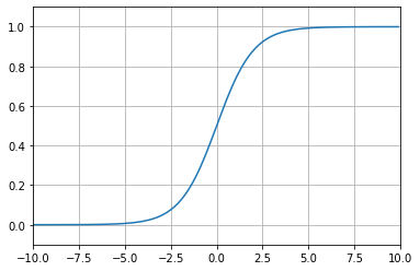
シグモイド関数
- ディープラーニングの基本的な技術であるニューラルネットワークでよく使われる
f(x) = \frac{1}{1 + e^{-x}}
対数関数
- 対数関数は、入力された値が底の何乗に相当するかを出力する
f(x) = \log_2 x
- 底がネイピア数(e)の時を特に自然対数と呼び、底のeが省略されたり、lnと書いたりすることがある
f(x) = \log x = \log_e x = \ln x
- 底が10の時は常用対数と呼ばれ、底の10が省略されることが時々ある
f(x) = \log x = \log_{10} x
-
底が省略されている場合、10なのかeなのかは注意が必要である
-
底が同じ対数同士の加算は乗算を行う
-
対数関数log xを微分して得られる値は以下の通り
(\log x)' = \frac{1}{x}
三角関数
- 三角関数:角度の大きさを入力とする関数
- sin(正弦)
- cos(余弦)
- tan(正接)
双曲線関数
\sinh{x} = \frac{e^x - e^{-x}}{2} \\

\cosh{x} = \frac{e^x + e^{-x}}{2} \\

\tanh{x} = \frac{\sinh{x}}{\cosh{x}}
■3.2.線形代数
ベクトルとその演算
ベクトルとは
- ベクトルとは、丸括弧で数をまとめて表現したもの
- ベクトルとの対比で、単なる1つの数をスカラーと呼ぶ
# ベクトル
(4, 7, 10, 12)
ノルム
- ノルムとは
- 英語で「標準、基準」などを意味する単語
- ベクトルの大きさをスカラーで表現すること
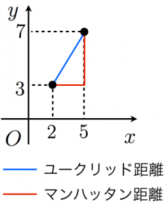
- ユークリッド距離:2点間の直線距離
2次元におけるユークリッド距離 = \sqrt{ {(x_1 - y_1)}^2 + {(x_2 - y_2)}^2}
- マンハッタン距離(L1距離):各座標の差(の絶対値)の総和を2点間の距離とする
2次元におけるマンハッタン距離 = | x_2 - x_1 | + | y_2 - y_1 |
- ユークリッド距離、マンハッタン距離どちらもnp.linalg.normで計算できる
import numpy as np
x1 = np.array([2, 3])
x2 = np.array([5, 7])

# ユークリッド距離
print(np.linalg.norm(x1 - x2))
# 5.0

# マンハッタン距離
print(np.linalg.norm(x1 - x2, ord=1))
# 7.0
行列とその演算
行列とは
- 行列(matrix)とは、行方向と列方向の2方向の広がりを持って数を並べたもの
- 正方行列:行と列のサイズが同じ行列
- 単位行列:正方行列のうち、左上から右下への対角線上にのる成分(対角成分)がすべて1で、残りの要素が0の行列
行列の演算
- 行列同士の足し算、引き算は、2つの行列の行数と列数が一致している必要がある
\begin{pmatrix}
a & b \\
c & d
\end{pmatrix}
+
\begin{pmatrix}
e & f \\
g & h
\end{pmatrix}
=
\begin{pmatrix}
a+e & b+f \\
c+g & d+h
\end{pmatrix}
- 行列の列の数とベクトルのサイズが同じ場合は、これらの掛け算を定義することができる
- 結果は元の行列の行数と同じサイズのベクトルとなる
\begin{pmatrix}
1 & 2 \\
3 & 4
\end{pmatrix}
\times
\begin{pmatrix}
5 \\
6
\end{pmatrix}
=
\begin{pmatrix}
1 \times 5 + 2 \times 6 \\
3 \times 5 + 4 \times 6
\end{pmatrix}
=
\begin{pmatrix}
17 \\
39
\end{pmatrix}
- 行列同士の掛け算は行列になる
- 数値の掛け算と違い、行列の掛け算は順番を入れ替えると結果が変わる場合がある
\begin{pmatrix}
1 & 2 \\
3 & 4
\end{pmatrix}
\times
\begin{pmatrix}
5 & 7 \\
6 & 8
\end{pmatrix}
=
\begin{pmatrix}
1 \times 5 + 2 \times 6 & 1 \times 7 + 2 \times 8 \\
3 \times 5 + 4 \times 6 & 3 \times 7 + 4 \times 8
\end{pmatrix}
=
\begin{pmatrix}
17 & 23 \\
39 & 53
\end{pmatrix}
・m \times sの行列に s \times nの行列を掛けると、m \times nの行列になるが、これを逆に考えると、m \times nの行列をm \times sの行列と s \times nの行列に分解できることになる
■3.3.基礎解析
微分と積分の意味
- 積分は面積
- 微分は傾き
- 関数F(x)を微分して、f(x)になる場合
- F:fの原始関数
- f:Fの導関数
- 偏微分:多変数関数の微分
■3.4.確率と統計
統計の基礎
- 代表値
- 最小値
- 最大値
- 平均値(mean):算術平均
- 中央値(median):
- 最頻値(mode)
- 分位数
- 四分位数
- ばらつきの指標
- 分散
- 標準偏差:分散の平方根
- 度数分布表
データの可視化方法
- ヒストグラム
- 箱ひげ図
- 散布図
データとその関係性
- 相関係数
- 共分散の値を、各変数の標準偏差の積で割ったものが相関係数となる
- 例:ある変数xの標準偏差が1、ある変数yの標準偏差が2、この2つのxとyの共分散が2であるとき、この2変数の相関係数は 2 / (1 * 2) = 1 となる
確率
- 条件付き確率
確率と分布
- 期待値
確率と関数
- 確率質量変数
- 確率密度変数
- 確率は確率密度関数の面積である。
- 正規分布
■4.ライブラリによる分析実践
■4.1.NumPy
4.1.1.概要
- 科学技術計算に特化したサードパーティ製パッケージ
- Pythonの標準型リストに比べて多次元配列のデータを効率よく扱える
- 配列用の型であるndarrayと行列用の型であるmatrixがある
- 配列や行列の要素のデータ型は一種類に揃える必要がある
import numpy as np
4.1.2.データを扱う
初期化
# 初期化
a1 = np.array([1, 2, 3]) # 1次元
a2 = np.array([[1, 2, 3], [4, 5, 6]]) # 2次元

print(a1)
# [1 2 3]
print(a2)
# [[1 2 3]
# [4 5 6]]

# オブジェクトの型を確認
print(type(a1))
# <class 'numpy.ndarray'>

# 配列の形状を確認
print(a1.shape)
# (3,)

print(a2.shape)
# (2, 3)
配列の形状を変換(reshape)
c1 = np.array([0, 1, 2, 3, 4, 5]) # 1次元
print(c1.shape)
# (6,)

c2 = c1.reshape((2, 3)) # 2行3列に変換
print(c2)
# [[0 1 2]
# [3 4 5]]

print(c2.shape)
# (2, 3)

# 要素数が合わないとエラーになる
c_err = c1.reshape((2, 4))
# ValueError: cannot reshape array of size 6 into shape (2,4)
多次元配列を1次元化する(ravel、flatten)
ravel、flattenどちらも同じ結果が得られる
# 使用するデータ
print(c2)
# [[0 1 2]
# [3 4 5]]

c3 = c2.ravel()
c4 = c2.flatten()

print(c3)
# [0 1 2 3 4 5]
print(c4)
# [0 1 2 3 4 5]
ravelとflattenの違い
- ravel:参照を返す
- flatten:コピーを返す(深いコピー)
c3[0] = 6
print(c3)
# [6 1 2 3 4 5]

# c2はc3変更の影響を受けている
print(c2)
# [[6 1 2]
# [3 4 5]]

c4[1] = 7
print(c4)
# [0 7 2 3 4 5]

# c2はc4変更の影響を受けていない
print(c2)
# [[6 1 2]
# [3 4 5]]
データ型(dtype)
# 作成時に型を宣言しないと自動で割り振られる
a = np.array([0, 1, 2])
print(a.dtype)
# int32

a = np.array([0.0, 1.0, 2.0])
print(a.dtype)
# float64

# 作成時に型宣言する
a = np.array([0, 1, 2], dtype=np.int16)
print(a.dtype)
# int16

a = np.array([0, 1, 2], dtype=np.float16)
print(a.dtype)
# float16
インデックス、スライスを使って配列から部分的にデータを取得する
# 使用するデータ
print(a1) # 1次元
# [10  2  3]
print(a2) # 2次元
# [[1 2 3]
# [4 5 6]]

# インデックス
print(a1[0]) # 最初の要素
# 10
print(a1[-1]) # 最後尾の要素
# 3
print(a2[1]) # 2行目
# [4 5 6]
print(a2[1, 0]) # 2行1列目の要素
# 4

# スライス
# 一次元
print(a1[1:]) # 2つ目含めそれ以降の要素
# [2 3]
print(a1[:1]) # 2つ目含めずそれ以前の要素
# [10]

# 多次元の場合は各次元のスライスをカンマで区切って指定
# つまり、二次元の場合は[行のスライス, 列のスライス] となる
# 先頭行の全列
print(a2[0:1, :])
# [[1 2 3]]
print(a2[0:1]) # 後ろの, : は省略できる
# [[1 2 3]]

# 全ての行の2つ目の要素
print(a2[:, 1:2])
# [[2]
# [5]]
print(a2[:, 1]) # スカラー値で指定すると一次元配列となる
# [2 5]
配列のコピー
# 使用するデータ
print(a1)
# [1 2 3]

a_refer = a1 # a1を参照するオブジェクトを生成(浅いコピー)
a_copy = a1.copy() # a1をコピーしたオブジェクトを生成(深いコピー)

print(a_refer)
# [1 2 3]
print(a_copy)
# [1 2 3]

a1[0] = 10
print(a1)
# [10  2  3]

# a1を参照するオブジェクトなので、a1の変更が反映される
print(a_refer)
# [10  2  3]

# a1をコピーしたオブジェクトなので、a1の変更は反映されない
print(a_copy)
# [1 2 3]
数列を作る
連番を生成(arange、linspace)
print(np.arange(10)) # 0 <= n < 10
# [0 1 2 3 4 5 6 7 8 9]
print(np.arange(1, 10)) # 1 <= n < 10
# [1 2 3 4 5 6 7 8 9]
print(np.arange(1, 10, 2)) # 1 <= n < 10 間隔:2
# [1 3 5 7 9]

print(np.linspace(1, 10, 7)) # 最初:1、最後:10 要素数:7
# [ 1.   2.5  4.   5.5  7.   8.5 10. ]
乱数を生成(rand、random、randint、uniform、randn)
np.random.seed(123) # 乱数のシード値を固定すると生成される値が固定される

# 一様分布(0.0 <= n < 1.0)
print(np.random.rand(3)) # 一次元
# [0.69646919 0.28613933 0.22685145]
print(np.random.rand(2, 3)) # 二次元
# [[0.55131477 0.71946897 0.42310646]
#  [0.9807642  0.68482974 0.4809319 ]]

# randomでも同じことができるが、配列サイズの渡し方が異なる
print(np.random.random(3)) # 一次元は同じ
# [0.39211752 0.34317802 0.72904971]
print(np.random.random((2, 3))) # 多次元の場合はタプルで渡す
# [[0.43857224 0.0596779  0.39804426]
#  [0.73799541 0.18249173 0.17545176]]
# 一様分布(任意の範囲の整数)
print(np.random.randint(1, 10)) # 1 <= n < 10
# 8
print(np.random.randint(1, 10, (2, 3))) # 1 <= n < 10 二次元配列(2 x 3)
# [[3 5 9]
#  [1 8 4]]
print(np.random.randint(1, 10, (3))) # 1 <= n < 10 一次元配列
# [5 7 2]

# 一様分布(任意の範囲の小数)
print(np.random.uniform(1, 5)) # 1.0 <= n < 5.0
# 3.6188852298792793
print(np.random.uniform(1, 5, (2, 3))) # 1.0 <= n < 5.0 二次元配列(2 x 3)
# [[2.49520571 1.9380515  4.95198115]
#  [4.0639838  4.10801776 1.11192782]]
print(np.random.uniform(1, 5, (3))) # 1.0 <= n < 5.0 一次元配列
# [1.69562606 1.61632897 1.30834592]
# 標準正規分布(平均0、分散1)
print(np.random.randn())
# 0.29822754810648927
print(np.random.randn(3)) # 一次元
# [0.46437133 0.11822163 1.94369786]
print(np.random.randn(2, 3)) # 二次元
# [[ 2.42320729 -1.26530807 -0.02627203]
#  [-1.92754197  0.56080222  0.24663925]]
同じ要素の配列を作る
print(np.zeros(3)) # 一次元
# [0. 0. 0.]
print(np.zeros((2, 3))) # 二次元
# [[0. 0. 0.]
#  [0. 0. 0.]]
print(np.ones(3)) # 一次元
# [1. 1. 1.]
print(np.ones((2, 3))) # 二次元
# [[1. 1. 1.]
#  [1. 1. 1.]]

# 指定値で埋める
print(np.full(3, 5)) # 一次元
# [5 5 5]
print(np.full((2, 3), 5)) # 二次元
# [[5 5 5]
#  [5 5 5]]
単位行列
print(np.eye(2))
# [[1. 0.]
#  [0. 1.]]
print(np.eye(3))
# [[1. 0. 0.]
#  [0. 1. 0.]
#  [0. 0. 1.]]
print(np.identity(3)) # eyeと同じ機能、使い方
# [[1. 0. 0.]
#  [0. 1. 0.]
#  [0. 0. 1.]]
配列操作
要素間の差分
d = np.array([2, 2, 7, 3, 8, -1])
print(np.diff(d))
# [ 0  5 -4  5 -9]
連結
a1 = np.full((2, 3), 2)
a2 = np.full((2, 3), 3)
print(a1)
# [[2 2 2]
#  [2 2 2]]
print(a2)
# [[3 3 3]
#  [3 3 3]]

# 行方向に連結
print(np.concatenate([a1, a2]))
# [[2 2 2]
#  [2 2 2]
#  [3 3 3]
#  [3 3 3]]
print(np.vstack([a1, a2])) # vstackも動作は同じ
# [[2 2 2]
#  [2 2 2]
#  [3 3 3]
#  [3 3 3]]

print(np.concatenate([a1, a2, np.full((2, 3), 4)])) # 連結する配列が3つ
# [[2 2 2]
#  [2 2 2]
#  [3 3 3]
#  [3 3 3]
# [4 4 4]
#  [4 4 4]]

# 列方向に連結
print(np.concatenate([a1, a2], axis=1)) # 2番目の次元(=2次元配列の場合は列)の方向に連結
# [[2 2 2 3 3 3]
#  [2 2 2 3 3 3]]
print(np.concatenate([a1, a2], 1)) # axisは省略可
# [[2 2 2 3 3 3]
#  [2 2 2 3 3 3]]
print(np.hstack([a1, a2])) # hstackも動作は同じ
# [[2 2 2 3 3 3]
#  [2 2 2 3 3 3]]
分割
a3 = np.concatenate([a1, a2])
print(a3)
# [[2 2 2]
#  [2 2 2]
#  [3 3 3]
#  [3 3 3]]

# 行方向に分割
a3_v1, a3_v2 = np.vsplit(a3, [1]) # 1つ目の配列が1行、2つ目が残りの行
print(a3_v1)
# [[2 2 2]]
print(a3_v2)
# [[2 2 2]
#  [3 3 3]
#  [3 3 3]]

# 列方向に分割
a3_h1, a3_h2 = np.hsplit(a3, [1]) # 1つ目の配列が1列、2つ目が残りの列
print(a3_h1)
# [[2]
#  [2]
#  [3]
#  [3]]
print(a3_h2)
# [[2 2]
#  [2 2]
#  [3 3]
#  [3 3]]
転置
print(a3)
# [[2 2 2]
#  [2 2 2]
#  [3 3 3]
#  [3 3 3]]

a3T = a3.T
print(a3T)
# [[2 2 3 3]
#  [2 2 3 3]
#  [2 2 3 3]]

print(a3T.shape)
# (3, 4)
print(a3.shape)
# (4, 3)
次元追加
a = np.array([1, 3, 5, 7])
print(a)
# [1 3 5 7]
print(a.shape)
# (4,)

a1 = a[np.newaxis, :] # 行方向に1つ次元を増やす
print(a1)
# [[1 3 5 7]]
print(a1.shape)
# (1, 4)

a2 = a[: ,np.newaxis ] # 列方向に1つ次元を増やす
print(a2)
# [[1]
#  [3]
#  [5]
#  [7]]
print(a2.shape)
# (4, 1)
グリッドデータの生成
x、y座標の配列から、それらを組み合わせてできるすべての点の座標データを生成する。
x = np.array([1, 2, 3, 4, 5])
y = np.array([6, 7, 8, 9, 10])
xx, yy = np.meshgrid(x, y)
print(xx)
# [[1 2 3 4 5]
#  [1 2 3 4 5]
#  [1 2 3 4 5]
#  [1 2 3 4 5]
#  [1 2 3 4 5]]
print(yy)
# [[ 6  6  6  6  6]
#  [ 7  7  7  7  7]
#  [ 8  8  8  8  8]
#  [ 9  9  9  9  9]
#  [10 10 10 10 10]]
4.1.3.各機能
ユニバーサルファンクション
配列要素内のデータを一括で変換してくれる。
# 絶対値:abs
a = np.array([1, -2, 3, -4, 5])
print(np.abs(a))
# [1 2 3 4 5]

# 角度→ラジアン変換:radians
b = np.radians([0, 15, 30, 45, 60, 75, 90])
print(b)
# [0.         0.26179939 0.52359878 0.78539816 1.04719755 1.30899694 1.57079633]

# 正弦:sin
print(np.sin(b))
# [0.         0.25881905 0.5        0.70710678 0.8660254  0.96592583 1.        ]

# 余弦:cos
print(np.cos(b))
# [1.00000000e+00 9.65925826e-01 8.66025404e-01 7.07106781e-01 5.00000000e-01 2.58819045e-01 6.12323400e-17]

# 正接:tan
print(np.tan(b))
# [0.00000000e+00 2.67949192e-01 5.77350269e-01 1.00000000e+00 1.73205081e+00 3.73205081e+00 1.63312394e+16]

# 自然対数:log
c = np.array([0, 1, 2, 3, np.e])
print(np.log(c))
# [      -inf 0.         0.69314718 1.09861229 1.        ]

# 常用対数:log10
d = np.array([0, 1, 2, 3, 10])
print(np.log10(d))
# [      -inf 0.         0.30103    0.47712125 1.        ]

# 指数関数(ネイピア数(e)のべき乗):exp
e = np.array([0, 1, 2])
print(np.exp(e))
# [1.         2.71828183 7.3890561 ]
ブロードキャスト
配列の内部データに直接演算などを行える機能。
# 配列と数値の演算
a = np.array([0, 1, 2])
print(a + 10)
# [10 11 12]

print(a - 10)
# [-10  -9  -8]

print(a * 2)
# [0 2 4]

print(a / 2)
# [0.  0.5 1. ]

print(a % 2)
# [0 1 0]

print(a ** 3)
# [0 1 8]
# 配列同士の演算
b = np.arange(-3, 3).reshape((2, 3))
print(a)
# [0 1 2]
print(b)
# [[-3 -2 -1]
#  [ 0  1  2]]

print(a + b)
# [[-3 -1  1]
#  [ 0  2  4]]

print(a - b)
# [[3 3 3]
#  [0 0 0]]

print(a * b)
# [[ 0 -2 -2]
#  [ 0  1  4]]

print(np.multiply(a, b)) # 行列同士の要素ごとの積
# [[ 0 -2 -2]
#  [ 0  1  4]]

print(a / b)
# [[-0.  -0.5 -2. ]
#  [ nan  1.   1. ]]
# ドット積
print(np.dot(b, a))
# [-4  5]

print(b @ a) # Python3.5以降で使える演算子でも同じ動作となる
# [-4  5]

print(np.matmul(b, a))
# [-4  5]
判定・論理値
配列と値を演算子で比較すると、比較結果の真偽値(True/False)が同じ形状の配列で出力される
b = np.arange(-3, 3).reshape((2, 3))
print(b)
# [[-3 -2 -1]
#  [ 0  1  2]]
print(b >= 1)
# [[False False False]
#  [False  True  True]]

# 条件に合致した要素を新たな配列として出力する
print(b[b >= 1])
# [1 2]

# 0ではない要素数を出力:count_nonzero
print(np.count_nonzero(b >= 1)) # False=0なのでTrueの数を出力している
# 2

# 要素の値を足す:sum
print(np.sum(b))
# -3
print(np.sum(b >= 1)) # True=1として計算される
# 2

# 要素の中にTrueが含まれているか:any
print(np.any(b >= 1))
# True
print(np.any(b > 10))
# False

# 要素全てがTrueか:all
print(np.all(b >= 1))
# False
print(np.all(b < 10))
# True

# 配列同士の比較も行える
print(a == b)
# [[False False False]
#  [ True  True  True]]

c = np.arange(1, 7).reshape((2, 3))
print(c)
# [[1 2 3]
#  [4 5 6]]

# 配列同士が同じ要素で構成されているか:allclose
print(np.allclose(b, c))
# False
print(np.allclose(b, c, atol=5)) # 誤差の範囲を指定できるので、浮動小数点計算の誤差を無視したい場合などに便利
# True
■4.2.pandas
4.2.1.概要
- Pythonでのデータ分析のツールとして最も活用されている
- Numpyを基盤にSeries(シリーズ)とDataFrame(データフレーム)というデータ型を提供している
import pandas as pd
# 辞書(dict)形式でDataFrameを初期化する
df = pd.DataFrame({'A' : [1, 2, 3], 'B' : [4, 5, 6], 'C' : ['a', 'b', 'c']}, index = ['line_1', 'line_2', 'line_3'])
print(df)
#         A  B  C
# line_1  1  4  a
# line_2  2  5  b
# line_3  3  6  c

# インデックス名、カラム名で抽出
print(df.loc['line_1', 'A'])
# 1

print(df.loc[:, 'A'])
# line_1    1
# line_2    2
# line_3    3
# Name: A, dtype: int64

print(df.loc[:, 'A':'B'])
#         A  B
# line_1  1  4
# line_2  2  5
# line_3  3  6

print(df.loc['line_1':'line_2', 'A':'B'])
#         A  B
# line_1  1  4
# line_2  2  5

# インデックス番号、カラム番号で抽出
print(df.iloc[0, 0])
# 1

print(df.iloc[:, 0])
# line_1    1
# line_2    2
# line_3    3
# Name: A, dtype: int64

print(df.iloc[:, 0:2])
#         A  B
# line_1  1  4
# line_2  2  5
# line_3  3  6

print(df.iloc[0:2, 0:2])
#         A  B
# line_1  1  4
# line_2  2  5
loc(インデックス名、カラム名での抽出)だと終端も含まれるけど、iloc(インデックス番号、カラム番号)は終端を含まない動作になっているもよう。
4.2.2.データの読み込み・書き込み
read_html:WebサイトのHTML内にあるtable要素を抜き出す
# WebサイトのHTML内にあるtable要素を抜き出す
df_html = pd.read_html('https://www.city.sapporo.jp/hokenjo/f1kansen/2019n-covhassei.html')

print(type(df_html))
# DataFrameのlistが返される
# <class 'list'>
print(len(df_html))
# 8

print(df_html[0].info())
# <class 'pandas.core.frame.DataFrame'>
# RangeIndex: 1 entries, 0 to 0
# Data columns (total 2 columns):
#  #   Column  Non-Null Count  Dtype
# ---  ------  --------------  -----
#  0   0       1 non-null      object
#  1   1       1 non-null      object
# dtypes: object(2)
# memory usage: 144.0+ bytes
# None

print(df_html[4])
#       0     1
# 0  陽性者数  259人
to_pickle:pandasのDataFrameをそのままファイルとして保存する(pickle形式に直列化して保存する)
read_pickle:pickle形式に直列化されたデータを読み込む
# pandasのDataFrameをそのままファイルとして保存する(pickle形式に直列化して保存する)
df.to_pickle('df.pkl')
print(df)
#         A  B  C
# line_1  1  4  a
# line_2  2  5  b
# line_3  3  6  c

print(df.info())
# <class 'pandas.core.frame.DataFrame'>
# Index: 3 entries, line_1 to line_3
# Data columns (total 3 columns):
#  #   Column  Non-Null Count  Dtype
# ---  ------  --------------  -----
#  0   A       3 non-null      int64
#  1   B       3 non-null      int64
#  2   C       3 non-null      object
# dtypes: int64(2), object(1)
# memory usage: 176.0+ bytes
# None

# pickle形式に直列化されたデータを読み込む
df_read = pd.read_pickle('df.pkl')

# 同じデータが同じ形式で保存されている
print(df_read)
#         A  B  C
# line_1  1  4  a
# line_2  2  5  b
# line_3  3  6  c

print(df_read.info())
# <class 'pandas.core.frame.DataFrame'>
# Index: 3 entries, line_1 to line_3
# Data columns (total 3 columns):
#  #   Column  Non-Null Count  Dtype
# ---  ------  --------------  -----
#  0   A       3 non-null      int64
#  1   B       3 non-null      int64
#  2   C       3 non-null      object
# dtypes: int64(2), object(1)
# memory usage: 96.0+ bytes
# None
4.2.3.データの整形
def judging_grades(score):
    if score < 60:
        return '3:可'
    elif score < 80:
        return '2:良'
    else:
        return '1:優'

df_score = pd.DataFrame({'国語' : [50, 70, 90]}, index = ['生徒A', '生徒B', '生徒C'])

# 列に関数を適用して新しい列を生成する
df_score.loc[:, '成績'] = df_score.loc[:, '国語'].apply(judging_grades)
print(df_score)
#      国語   成績
# 生徒A  50  3:可
# 生徒B  70  2:良
# 生徒C  90  1:優

# カテゴリ変数をダミー変数に変換
df_score = pd.get_dummies(df_score.loc[:, '成績'], prefix='成績(国語)')
print(df_score)
#      成績(国語)_1:優  成績(国語)_2:良  成績(国語)_3:可
# 生徒A           0           0           1
# 生徒B           0           1           0
# 生徒C           1           0           0
- pandas.Series.value_counts()
- ユニークな要素の値がindex、その出現個数がdataとなるpandas.Seriesを返す
- pandas.Series.to_frame()
- SeriesをDataFrameに変換する
4.2.4.時系列データ
pandas.date_range()で、datetime64[ns]型のインデックスであるDatetimeIndexを生成する。
# 指定した期間
df_index = pd.date_range(start='2022-04-01', end='2022-04-10')
print(df_index)
# DatetimeIndex(['2022-04-01', '2022-04-02', '2022-04-03', '2022-04-04',
#                '2022-04-05', '2022-04-06', '2022-04-07', '2022-04-08',
#                '2022-04-09', '2022-04-10'],
#               dtype='datetime64[ns]', freq='D')

# 生成したインデックスからDataFrameを作成
np.random.seed(123)
df = pd.DataFrame(np.random.randint(1, 11, 10), index=df_index, columns=['乱数'])
print(df)
#             乱数
# 2022-04-01   3
#2022-04-02   3
(中略)
# 2022-04-09   1
# 2022-04-10   2
# 指定した日数
print(pd.date_range(start='2022-04-01', periods=10))
# DatetimeIndex(['2022-04-01', '2022-04-02', '2022-04-03', '2022-04-04',
#                '2022-04-05', '2022-04-06', '2022-04-07', '2022-04-08',
#                '2022-04-09', '2022-04-10'],
#               dtype='datetime64[ns]', freq='D')
# 指定期間の指定頻度
# 毎週日曜
print(pd.date_range(start='2022-04-01', end='2022-04-30', freq='W'))
# DatetimeIndex(['2022-04-03', '2022-04-10', '2022-04-17', '2022-04-24'], dtype='datetime64[ns]', freq='W-SUN')

# 毎週土曜
print(pd.date_range(start='2022-04-01', end='2022-04-30', freq='W-SAT'))
# DatetimeIndex(['2022-04-02', '2022-04-09', '2022-04-16', '2022-04-23',
#                '2022-04-30'],
#               dtype='datetime64[ns]', freq='W-SAT')
- freq='W'とすると毎週日曜日の日付が選択される
- freq='W-SAT'のようにすることで毎週指定曜日の日付が選択される
- W-SUN(Wと同じ), W-MON, W-TUE, W-WED, W-THU, W-FRI, W-SAT
# 月ごとの平均値を出す
df_index = pd.date_range(start='2022-01-01', periods=365)
np.random.seed(123)
df = pd.DataFrame(np.random.randint(1, 366, 365), index=df_index, columns=['乱数'])
print(df.groupby(pd.Grouper(freq='M')).mean())
#                     乱数
# 2022-01-31  162.225806
# 2022-02-28  214.321429
(中略)
# 2022-11-30  158.166667
# 2022-12-31  207.322581

# DataFrame.resample()でも同じことが行える
print(df.loc[:, '乱数'].resample('M').mean())
# 2022-01-31  162.225806
# 2022-02-28  214.321429
(中略)
# 2022-11-30  158.166667
# 2022-12-31  207.322581
# Freq: M, Name: 乱数, dtype: float64
- pandas.Grouper で周期的なグルーピングを行うことができる
- freq='M'とすることで月ごとのデータ、'W'とすることで週ごとのデータがグルーピングされる
4.2.5.欠損値処理
df = pd.DataFrame({"A":[1,2,np.nan,4,5], "B":[6,np.nan,8,9,10]})
print(df)
#      A     B
# 0  1.0   6.0
# 1  2.0   NaN
# 2  NaN   8.0
# 3  4.0   9.0
# 4  5.0  10.0

# 欠損値を0で補完
print(df.fillna(0))
#      A     B
# 0  1.0   6.0
# 1  2.0   0.0
# 2  0.0   8.0
# 3  4.0   9.0
# 4  5.0  10.0

# 欠損値を1つ手前の値で補完
print(df.fillna(method='ffill')) # ffillの代わりにbfillを与えると1つ後ろの値で補完される
#      A     B
# 0  1.0   6.0
# 1  2.0   6.0
# 2  2.0   8.0
# 3  4.0   9.0
# 4  5.0  10.0

# 欠損値を平均値で補完
print(df.fillna(df.mean()))
#      A      B
# 0  1.0   6.00
# 1  2.0   8.25
# 2  3.0   8.00
# 3  4.0   9.00
# 4  5.0  10.00
4.2.6.データ連結
df1 = pd.DataFrame({"A":[1,2,3,4,5], "B":[6,7,8,9,10]})
df2 = pd.DataFrame({"A":[1,2,3,4,5], "B":[6,7,8,9,10]})
df3 = pd.DataFrame({"C":[1,2,3,4,5], "D":[6,7,8,9,10]})
# 行方向の連結
print(pd.concat([df1, df2]))
#    A   B
# 0  1   6
# 1  2   7
# 2  3   8
# 3  4   9
# 4  5  10
# 0  1   6
# 1  2   7
# 2  3   8
# 3  4   9
# 4  5  10

# 列方向の連結
print(pd.concat([df1, df3], axis=1))
#    A   B  C   D
# 0  1   6  1   6
# 1  2   7  2   7
# 2  3   8  3   8
# 3  4   9  4   9
# 4  5  10  5  10
pandasでのmergeとjoinの違い
- join()はmerge()のようにpandas.join()関数は用意されておらず、pandas.DataFrameのメソッドだけである
- 内部結合(how='inner')がデフォルトのmerge()とは異なり、join()は左結合(how='left')がデフォルト
- 呼び出し元のpandas.DataFrameのキーとする列を引数onで指定できるが、引数に指定する側のpandas.DataFrameは常にインデックスがキーとなる
4.2.7.統計データの扱い
df_index = pd.date_range(start='2022-04-01', end='2022-04-10')
np.random.seed(123)
df = pd.DataFrame(np.random.randint(1, 11, 10), index=df_index, columns=['乱数'])
print(df)
#             乱数
# 2022-04-01   3
# 2022-04-02   3
# 2022-04-03   7
# 2022-04-04   2
# 2022-04-05   4
# 2022-04-06  10
# 2022-04-07   7
# 2022-04-08   2
# 2022-04-09   1
# 2022-04-10   2

# 最大値
print(df.loc[:, '乱数'].max())
# 10

# 最小値
print(df.loc[:, '乱数'].min())
# 1

# 最頻値
print(df.loc[:, '乱数'].mode())
# 0    2
# dtype: int32

# 算術平均(平均値)
print(df.loc[:, '乱数'].mean())
# 4.1

# 中央値
print(df.loc[:, '乱数'].median())
# 3.0

# 標準偏差(標本標準偏差)
print(df.loc[:, '乱数'].std())
# 2.923088169119167

# 母集団の標準偏差
print(df.loc[:, '乱数'].std(ddof=0))
# 2.773084924772409

# DataFrameをNumpyの配列(ndarray)に変換する
print(df.loc[:, '乱数'].values)
# [ 3  3  7  2  4 10  7  2  1  2]
■4.3.Matplotlib
4.3.1.概要
- Pythonで主に2次元のグラフを描画するためのライブラリ
- グラフを描画するコードに2つのスタイルがある
- MATLABスタイル
- オブジェクト指向スタイル
import matplotlib.pyplot as plt
4.3.2.描画オブジェクト
import matplotlib.pyplot as plt
import matplotlib.style
# グラフの表示スタイル一覧を表示
print(matplotlib.style.available)
# ['Solarize_Light2', '_classic_test_patch', 'bmh', 'classic', 'dark_background', 'fast', 'fivethirtyeight', 'ggplot', 'grayscale', 'seaborn', 'seaborn-bright', 'seaborn-colorblind', 'seaborn-dark', 'seaborn-dark-palette', 'seaborn-darkgrid', 'seaborn-deep', 'seaborn-muted', 'seaborn-notebook', 'seaborn-paper', 'seaborn-pastel', 'seaborn-poster', 'seaborn-talk', 'seaborn-ticks', 'seaborn-white', 'seaborn-whitegrid', 'tableau-colorblind10']
# 表示スタイルを指定
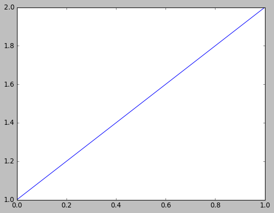
matplotlib.style.use('classic')
fig, ax = plt.subplots()
ax.plot([1, 2])
plt.show()
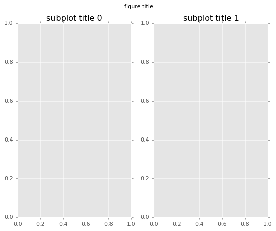
import matplotlib.pyplot as plt

fig, ax = plt.subplots(ncols=2)
# サブプロットにタイトルを設定
ax[0].set_title('subplot title 0')
ax[1].set_title('subplot title 1')
# 描画オブジェクトにタイトルを設定
fig.suptitle('figure title')

plt.show()
4.3.3.グラフの種類と出力方法
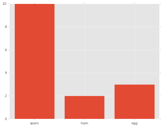
import matplotlib.pyplot as plt

fig, ax = plt.subplots()

x = [1, 2, 3]
y = [10, 2, 3]
labels = ['spam', 'ham', 'egg']

# 棒グラフ
ax.bar(x, y, tick_label=labels)

plt.show()
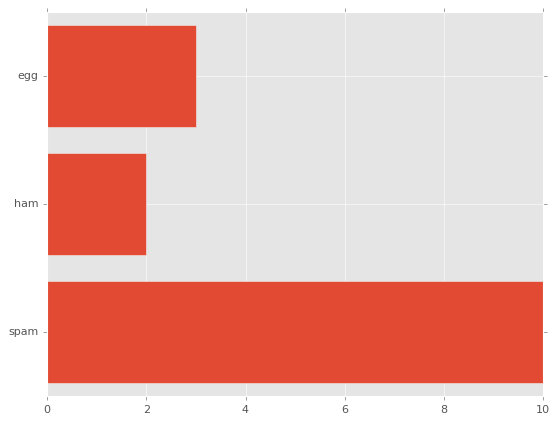
import matplotlib.pyplot as plt

fig, ax = plt.subplots()

x = [1, 2, 3]
y = [10, 2, 3]
labels = ['spam', 'ham', 'egg']

# 横向きの棒グラフ
ax.barh(x, y, tick_label=labels)

plt.show()
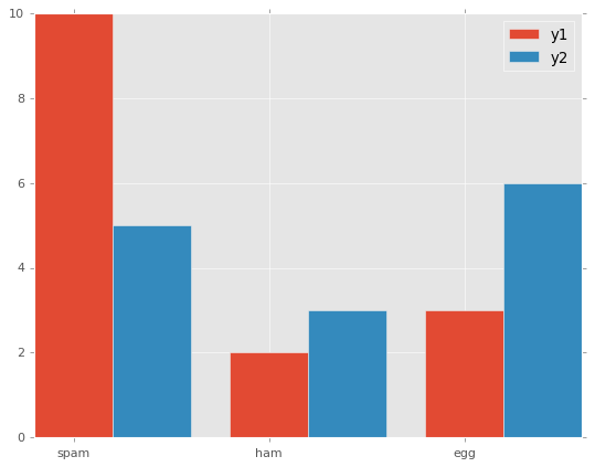
# 2つのデータの棒グラフを描画
import matplotlib.pyplot as plt

fig, ax = plt.subplots()

x = [1, 2, 3]
y1 = [10, 2, 3]
y2 = [5, 3, 6]
labels = ['spam', 'ham', 'egg']

width = 0.4 # 棒グラフの幅

ax.bar(x, y1, width=width, tick_label=labels, label='y1') # 幅を指定して描画

# 幅分ずらして棒グラフを描画
x2 = [num + width for num in x]
ax.bar(x2, y2, width=width, label='y2')

ax.legend()

plt.show()
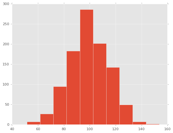
import matplotlib.pyplot as plt
import numpy as np

# データを生成
np.random.seed(123)
# 平均:100、標準偏差:15の正規分布に従う乱数を1,000個定義
x = np.random.normal(100, 15, 1000)

fig, ax = plt.subplots()

# ヒストグラムを描画
# 戻り値:各ビンの度数、各ビンの範囲、パッチオブジェクトが格納されている配列
n, bins, patches = ax.hist(x)

# 戻り値は度数分布表に使用できる値
for i, num in enumerate(n):
    print('{:.2f} - {:.2f}: {}'.format(bins[i], bins[i + 1], num))

# 51.53 - 61.74: 7.0
# 61.74 - 71.94: 27.0
# 71.94 - 82.15: 95.0
# 82.15 - 92.35: 183.0
# 92.35 - 102.55: 286.0
# 102.55 - 112.76: 202.0
# 112.76 - 122.96: 142.0
# 122.96 - 133.17: 49.0
# 133.17 - 143.37: 7.0
# 143.37 - 153.57: 2.0

plt.show()
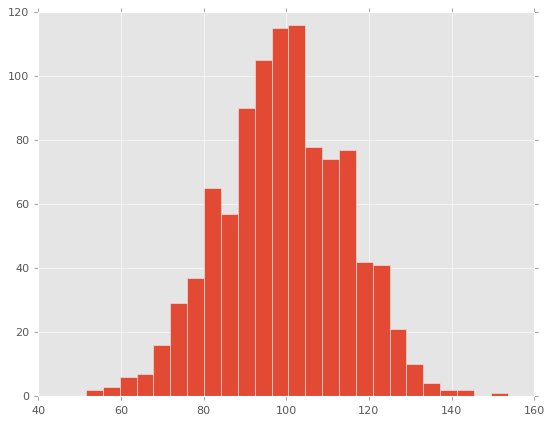
fig, ax = plt.subplots()

# ヒストグラムを描画
ax.hist(x, bins=25) # ピンの数を指定(未指定時は10)

plt.show()
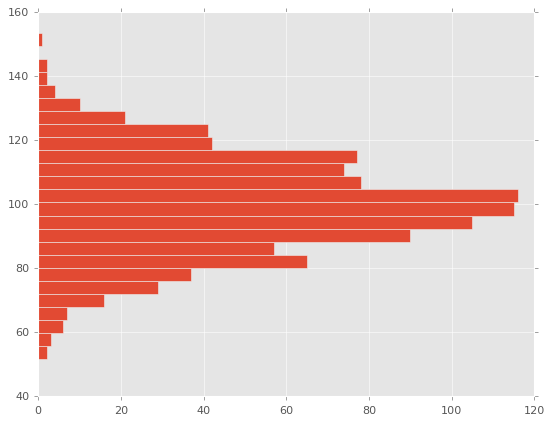
fig, ax = plt.subplots()

# ヒストグラムを描画
ax.hist(x, bins=25, orientation='horizontal') # 横向きで表示

plt.show()
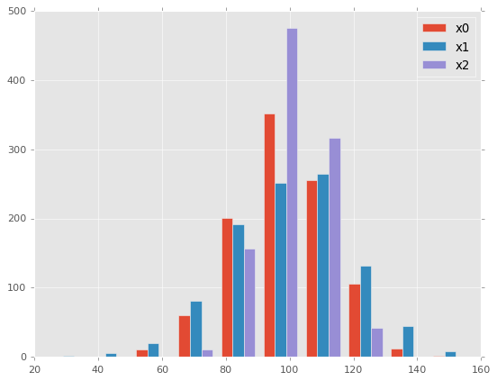
import matplotlib.pyplot as plt
import numpy as np

# データを生成
np.random.seed(123)
x0 = np.random.normal(100, 15, 1000)
x1 = np.random.normal(100, 20, 1000)
x2 = np.random.normal(100, 10, 1000)

fig, ax = plt.subplots()

labels = ['x0', 'x1', 'x2']
# 3つのデータのヒストグラムを描画
# ヒストグラムでは棒グラフと異なり、複数の値を指定すると自動的に横に並べて表示してくれる
ax.hist((x0, x1, x2),label=labels)
ax.legend()

plt.show()
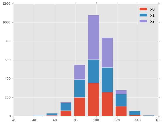
fig, ax = plt.subplots()

labels = ['x0', 'x1', 'x2']
# 3つのデータの積み上げたヒストグラムを描画
ax.hist((x0, x1, x2),label=labels, stacked=True)
ax.legend()

plt.show()
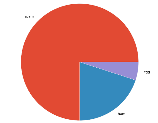
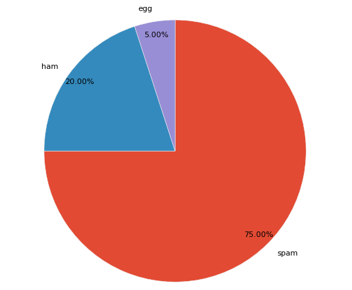
import matplotlib.pyplot as plt

labels = ['spam', 'ham', 'egg']
x = [75, 20, 5]

fig, ax = plt.subplots()
ax.pie(x, labels=labels) # 円グラフを描画
ax.axis('equal') # アスペクト比を保持して(円のままで)描画する

plt.show()
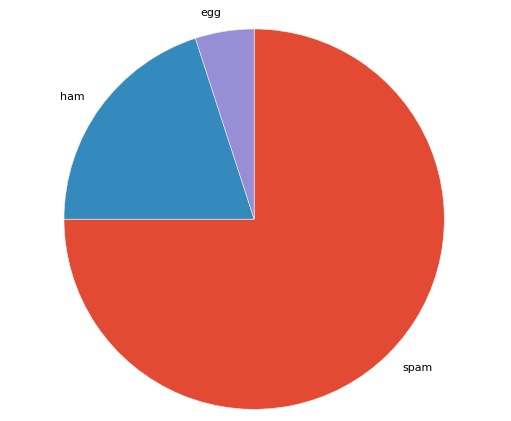
fig, ax = plt.subplots()
ax.pie(x, labels=labels, startangle=90, counterclock=False) # 上から時計回りに描画
ax.axis('equal')

plt.show()
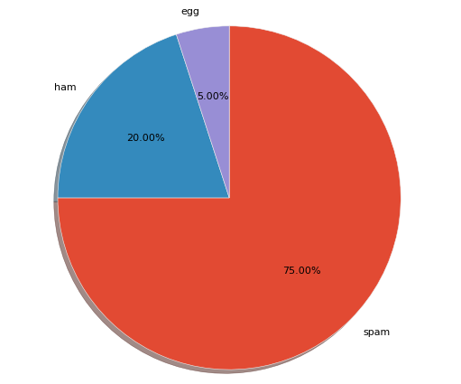
fig, ax = plt.subplots()
ax.pie(x, labels=labels, startangle=90, counterclock=False
        , shadow=True, autopct='%1.2f%%') # 影と%表記を追加
ax.axis('equal')

plt.show()
fig, ax = plt.subplots()
ax.pie(x, labels=labels, startangle=90, counterclock=False
        , autopct='%1.2f%%', pctdistance=0.9) # %表記の位置指定(デフォルト値:0.6)
ax.axis('equal')

plt.show()
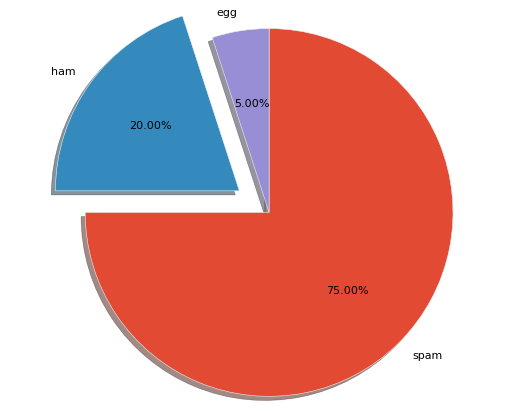
fig, ax = plt.subplots()
ax.pie(x, labels=labels, startangle=90, counterclock=False
        , shadow=True, autopct='%1.2f%%'
        , explode=[0, 0.2, 0]) # 2番目の要素を切り出す
ax.axis('equal')

plt.show()
4.3.4.スタイル
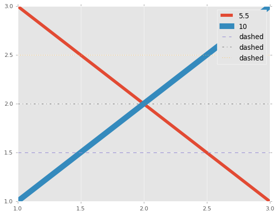
import matplotlib.pyplot as plt

fig, ax = plt.subplots()

# 線幅
ax.plot([1, 3], [3, 1], linewidth=5.5, label='5.5')
ax.plot([1, 3], [1, 3], linewidth=10, label='10')
# 線の種類
ax.plot([1, 3], [1.5, 1.5], linestyle='--', label='dashed') # 破線
ax.plot([1, 3], [2, 2], linestyle='-.', label='dashed') # 一点鎖線
ax.plot([1, 3], [2.5, 2.5], linestyle=':', label='dashed') # 点線

ax.legend()

plt.show()
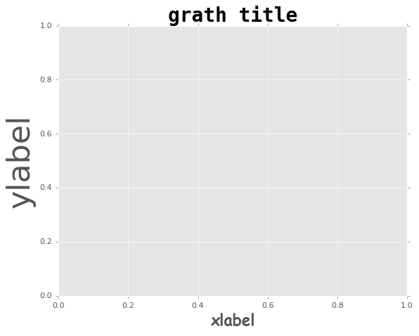
fig, ax = plt.subplots()

# フォントの種類・太さ
ax.set_xlabel('xlabel', family='fantasy', size=20, weight='bold')
ax.set_ylabel('ylabel', family='sans-serif', size=40, weight='light')
ax.set_title('grath title', family='monospace', size=25, weight='heavy')

plt.show()
# フォントのスタイルを辞書で定義
fontdict = {
    'family' : 'fantasy'
    ,'color' : 'black'
    ,'weight' : 'normal'
    ,'size' : 20
}

fig, ax = plt.subplots()

ax.set_xlabel('xlabel', fontdict=fontdict)
ax.set_ylabel('ylabel', fontdict=fontdict)
ax.set_title('grath title', fontdict=fontdict, size=40) # sizeのみ個別指定で上書き

plt.show()
■4.4.scikit-learn
4.4.1.前処理
import numpy as np
import pandas as pd

# サンプルのデータセットを作成
df = pd.DataFrame(
    {
        'A' : [1, np.nan, 3, 4, 5]
        ,'B' : [6, 7, 8, np.nan, 10]
        ,'C' : [11, 12, 13, 14, 15]
    }
)

df
#   A	B	C
# 0	1.0	6.0	11
# 1	NaN	7.0	12
# 2	3.0	8.0	13
# 3	4.0	NaN	14
# 4	5.0	10.0	15
欠損値の補完:SimpleImputer
from sklearn.impute import SimpleImputer
# 平均値で欠損値を補完するインスタンスを作成する
imp = SimpleImputer(strategy='mean')
# 平均値で欠損値を補完
imp.fit(df)
imp.transform(df)
# array([[ 1.  ,  6.  , 11.  ],
#        [ 3.25,  7.  , 12.  ],
#        [ 3.  ,  8.  , 13.  ],
#        [ 4.  ,  7.75, 14.  ],
#        [ 5.  , 10.  , 15.  ]])
カテゴリ変数のエンコーディング:LabelEncoder
- 「a→0, b→1, c→2」のようにカテゴリ変数を数値に変換する処理を指す
# サンプルのデータセットを作成
df = pd.DataFrame(
    {
        'A' : [1, 2, 3, 4, 5]
        ,'B' : ['a', 'b', 'a', 'b', 'c']
    }
)

df
# 	A	B
# 0	1	a
# 1	2	b
# 2	3	a
# 3	4	b
# 4	5	c
from sklearn.preprocessing import LabelEncoder
# ラベルエンコーダのインスタンスを作成
le = LabelEncoder()
# ラベルのエンコーディング
le.fit(df['B'])
print(le.transform(df['B']))
# [0 1 0 1 2]

# 元の値を確認
print(le.classes_)
# ['a' 'b' 'c']
One-hotエンコーディング:ColumnTransformer
- カテゴリ変数に対して行う符号化の処理
- 取り得る値の分だけ列を増やして、各行の該当する値の列のみに1が、それ以外の列には0が入力される
from sklearn.preprocessing import LabelEncoder, OneHotEncoder
from sklearn.compose import ColumnTransformer

df_one = df.copy()
print(df_one)
#    A  B
# 0  1  a
# 1  2  b
# 2  3  a
# 3  4  b
# 4  5  c

# One-hotエンコーディングのインスタンス化
one = ColumnTransformer([('OneHotEncoder', OneHotEncoder(), [1])], remainder='passthrough')
# One-hotエンコーディング
one.fit_transform(df_one)
# array([[1., 0., 0., 1.],
#        [0., 1., 0., 2.],
#        [1., 0., 0., 3.],
#        [0., 1., 0., 4.],
#        [0., 0., 1., 5.]])
分散正規化:StandardScaler
- 特徴量の平均が0、標準偏差が1となるように特徴量を変換する処理
# サンプルのデータセットを作成
df = pd.DataFrame(
    {
        'A' : [1, 2, 3, 4, 5]
        ,'B' : [100, 200, 400, 500, 800]
    }
)

df
# 	A	B
# 0	1	100
# 1	2	200
# 2	3	400
# 3	4	500
# 4	5	800
from sklearn.preprocessing import StandardScaler
# 分散正規化のインスタンスを作成
stdsc = StandardScaler()
# 分散正規化を実行
stdsc.fit(df)
stdsc.transform(df)
# array([[-1.41421356, -1.22474487],
#        [-0.70710678, -0.81649658],
#        [ 0.        ,  0.        ],
#        [ 0.70710678,  0.40824829],
#        [ 1.41421356,  1.63299316]])
最小最大正規化:MinMaxScaler
- 特徴量の最小値が0、最大値が1をとるように特徴量を正規化する処理
from sklearn.preprocessing import MinMaxScaler
# 最小最大正規化のインスタンスを作成
mmsc = MinMaxScaler()
# 最小最大正規化を実行
mmsc.fit(df)
mmsc.transform(df)
# array([[0.        , 0.        ],
#        [0.25      , 0.14285714],
#        [0.5       , 0.42857143],
#        [0.75      , 0.57142857],
#        [1.        , 1.        ]])
4.4.2.分類
サポートベクタマシン
- 分類・回帰及び外れ値検出に使えるアルゴリズム
- 直線や平面で線形分離できないデータを高次元の空間に写して線形分離することにより分類を行うアルゴリズム
- 実際には高次元の空間に写すのではなく、データ間の近さを定量化するカーネルを導入している
- svmモジュールのSVCクラスを使用する
- アルゴリズムとしては以下の通り
- 分類したいクラスのデータ間に直線(決定境界)を引く
- この直線は、各クラスのデータ(サポートベクタ)間の距離が最も大きくなるように引く
- クラス間のサポートベクタの距離をマージンと呼ぶ
- 極端に絶対値の大きな特徴量に分類結果が影響を受けやすい傾向がある
- 正規化を行い、それぞれの特徴量の尺度を揃えておくとよい
- カーネルをrbfカーネルなどにすることで非線形構造を有するデータに対しても使用することができる
- scikit-learnで使用する場合、カーネルはガウスカーネル以外にも指定することができる
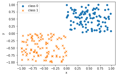
import numpy as np
import matplotlib.pyplot as plt

np.random.seed(123)
# クラス0:X軸Y軸ともに0~1までの一様分布から100点をサンプリング
X0 = np.random.uniform(size=(100, 2))
# クラス0のラベルを100個生成
y0 = np.repeat(0, 100)
# クラス1:X軸Y軸ともに-1~0までの一様分布から100点をサンプリング
X1 = np.random.uniform(-1.0, 0.0, size=(100, 2))
# クラス1のラベルを100個生成
y1 = np.repeat(1, 100)

# 散布図にプロット
fig, ax = plt.subplots()
ax.scatter(X0[:, 0], X0[:, 1], marker='o', label='class 0')
ax.scatter(X1[:, 0], X1[:, 1], marker='x', label='class 1')
ax.set_xlabel('x')
ax.set_ylabel('y')
ax.legend()
plt.show()
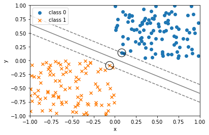
from sklearn.svm import SVC

# サポートベクタマシンのインスタンス化
# Cの値が小さいほど、マージンは大きくなる
svc = SVC(kernel='linear', C=1e6)
# 学習
svc.fit(np.vstack((X0, X1)), np.hstack((y0, y1)))

fig, ax = plt.subplots()
ax.scatter(X0[:, 0], X0[:, 1], marker='o', label='class 0')
ax.scatter(X1[:, 0], X1[:, 1], marker='x', label='class 1')

# 決定境界とマージンをプロット
xx, yy = np.meshgrid(np.linspace(-1, 1, 100), np.linspace(-1, 1, 100))
xy = np.vstack([xx.ravel(), yy.ravel()]).T # -1~1までを100分割したx, yの全組み合わせ
p = svc.decision_function(xy).reshape((100, 100))
# 等高線をプロット
ax.contour(xx, yy, p,
            colors='k', levels=[-1, 0, 1],
            alpha=0.5, linestyles=['--', '-', '--'])

# サポートベクタをプロット
# グラフ的にはすでにプロットしているデータに丸で印をつけている格好となる
ax.scatter(svc.support_vectors_[:, 0],
            svc.support_vectors_[:, 1],
            s=250, facecolors='none',
            edgecolors='black')


ax.set_xlabel('x')
ax.set_ylabel('y')
ax.legend(loc='best')
plt.show()
決定木
- データを分割するルールを次々と作成していくことにより、分類を実行するアルゴリズム
- 「ノード」とそれらを結ぶ「エッジ」から構成される
- 木の最上部にあり親ノードを持たないノードは根ノードと呼ばれる
- 木の最下部にあり子ノードを持たないノードは葉ノードと呼ばれる
- データを分割する基準は、どれだけクラスが混在しているかを示す不純度が下がることから判断していく
- 親ノードの不純度から子ノードの不純度の合計を引いた値を情報利得と呼び、これが正の値になるように分割していく
- 情報利得の大きい順に特徴量が使用され、木が作られる
- 不純度の指標として、ジニ不純度、エントロピー、分類誤差などがある(情報利得は含まれない)
- ジニ不純度:各ノードに間違ったクラスが振り分けられてしまう確率
- treeモジュールのDecisionTreeClassifierクラスを使用する
- 木の数は引数として指定できない
- ある2つのカテゴリー(ラベル0とラベル1)を持つ特徴量を分割する場合のジニ不純度は、ラベル0なのにラベル1と割り振られる確率とラベル1なのにラベル0と割り振られる確率の和を考える必要がある
- クラス0である確率をP(0)、クラス1である確率をP(1)とすると、求めるジニ不純度は以下の通りとなる
ジニ不純度 = 1 - (P(0)^2 + P(1)^2)
from sklearn.datasets import load_iris
from sklearn.model_selection import train_test_split
from sklearn.tree import DecisionTreeClassifier

# Irisデータセットを読み込む
iris = load_iris()
X, y = iris.data, iris.target
# 学習データセットとテストデータセットに分割する
X_train, X_test, y_train, y_test = train_test_split(X, y, test_size=0.3, random_state=123)
# 決定木をインスタンス化する(木の最大の深さ=3)
tree = DecisionTreeClassifier(max_depth=3)
# 学習
tree.fit(X_train, y_train)
# 予測
y_pred = tree.predict(X_test)
print(y_pred)
# [1 2 2 1 0 1 1 0 0 1 2 0 1 2 2 2 0 0 1 0 0 1 0 2 0 0 0 2 2 0 2 1 0 0 1 1 2 0 0 1 1 0 2 2 2]
ランダムフォレスト
- データの説明変数となる特徴量をランダムに選択して決定機を構築する処理を複数回繰り返し、各木の推定結果の多数決や平均値により分類・回帰を行う手法
- 他の機械学習アルゴリズムと比較すると、欠損値の穴埋めや標準化などのデータの前処理を必要としないアルゴリズムである
- ランダムに選択された特徴量をブートストラップデータと呼ぶ
- ランダムフォレストのように、複数の学習器を用いた学習はアンサンブル学習と呼ばれる
- ensembleモジュールのRandomForestClassfierクラスを使用する
# ランダムフォレスト
from sklearn.ensemble import RandomForestClassifier

# ランダムフォレストをインスタンス化する(決定木の個数=100)
# この例では指定していないが、決定木と同様にmax_depthで木の最大の深さを指定できる
forest = RandomForestClassifier(n_estimators=100, random_state=123)
# 学習
forest.fit(X_train, y_train)
# 予測
y_pred = forest.predict(X_test)
print(y_pred)
# [1 2 2 1 0 1 1 0 0 1 2 0 1 2 2 2 0 0 1 0 0 1 0 2 0 0 0 2 2 0 2 1 0 0 1 1 2 0 0 1 1 0 2 2 2]
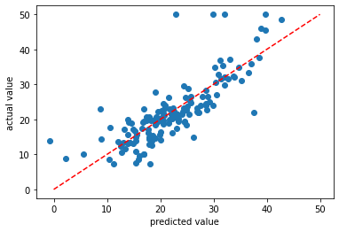
4.4.3.回帰
- ある値(目的変数)を別の単一または複数の値(説明変数、特徴量)で説明するタスク
- 説明変数が1つの場合を単回帰、2つ以上の場合を重回帰と呼ぶ
- linear_modelモジュールのLinearRegressionクラスを使用する
- 線形回帰の損失関数に対しての正則化項
- Ridge回帰:L2正則化項
- Lasso回帰:L1正則化項
from sklearn.linear_model import LinearRegression
from sklearn.datasets import load_boston
from sklearn.model_selection import train_test_split

# Bostonデータセットを読み込む
boston = load_boston()
X, y = boston.data, boston.target
# 学習データセットとテストデータセットに分割
X_train, X_test, y_train, y_test = train_test_split(X, y, test_size=0.3, random_state=123)
# 線形回帰をインスタンス化
lr = LinearRegression()
# 学習
lr.fit(X_train, y_train)
# テストデータセットを予測
y_pred = lr.predict(X_test)
print(y_pred)
# [15.4757088  27.85786595 39.71821366 17.94591734 30.19441873  37.51057831 25.20492485 11.29301795 13.93325033 32.10798674 28.51346127 19.10242965 14.16909335 30.59883198 16.91765089 21.57521646 20.56956106 38.0388848
# ・・・
# 横軸を予測値、縦軸を実績値とする散布図をプロットする
import matplotlib.pyplot as plt

fig, ax = plt.subplots()
ax.scatter(y_pred, y_test)
# y=xの直線をプロットする
ax.plot((0, 50), (0, 50), linestyle='dashed', color='red')
ax.set_xlabel('predicted value')
ax.set_ylabel('actual value')
plt.show()
4.4.4.次元削減
- データが持っている情報をなるべく損ねることなく次元を削減してデータを圧縮するタスク
- 機械学習においては、計算時間の短縮を主目的として使われる
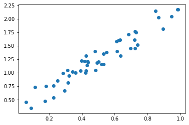
主成分分析(PCA)
- 次元削減の手法の一つ
- 高次元のデータに対して、分散が大きくなる(データが散らばっている)方向を探して、元の次元と同じかそれよりも低い次元にデータを変換する手法
- decompositionモジュールのPCAクラスを使用する
import numpy as np
import matplotlib.pyplot as plt

np.random.seed(123)
# x軸:0以上1未満の一様乱数を50個生成
X = np.random.rand(50)
# y軸:Xを2倍した後に、0以上1未満の一様乱数を0.5倍して足し合わせる
Y = 2 * X + 0.5 * np.random.rand(50)
# 散布図をプロット
fig, ax = plt.subplots()
ax.scatter(X, Y)
plt.show()
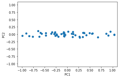
from sklearn.decomposition import PCA
# 主成分のクラスをインスタンス化
pca = PCA(n_components=2)
# 主成分分析を実行
X_pca = pca.fit_transform(np.hstack((X[:, np.newaxis], Y[:, np.newaxis])))
# 主成分分析の結果得られた座標を散布図にプロット
fig, ax = plt.subplots()
ax.scatter(X_pca[:, 0], X_pca[:, 1])
ax.set_xlabel('PC1')
ax.set_ylabel('PC2')
ax.set_xlim(-1.1, 1.1)
ax.set_ylim(-1.1, 1.1)
plt.show()
4.4.5.モデルの評価
カテゴリの分類精度
- 混同行列:予測と実績のクラスラベルの組合せを集計した表
| 実績:正例 | 実績:負例 | |
|---|---|---|
| 予測:正例 | TP:正例と予測して実際に正例 | FP:正例と予測したが実際は負例 |
| 予測:負例 | FN:負例と予測したが実際は正例 | TN:負例と予測して実際に負例 |
-
適合率(precision)
- 正例(負例)と予測したデータの内、実際に正例(負例)の割合を示す
- TP / (TP + FP) または FN / (FN + TN)
-
再現率(recall)
- 実際の正例(負例)の内、正例(負例)と予測したものの割合を示す
- TP / (TP + FN) または TN / (TN + FP)
-
F値(F-Value)
- 適合率と再現率の調和平均
- 2 * 適合率 * 再現率 / (適合率 + 再現率)
- 適合率と再現率はトレードオフの関係にある(どちらかを高くするともう一方は低くなる)
- 適合率と再現率両方の指標がバランスの良い値になることを目指すときに重視する指標
-
正解率(accuracy)
- 正例、負例を問わず、予測と実績が一致したデータの割合を示す
- (TP + TN) / (TP + FP + FN + TN)
-
scikit-learnのmetricモジュールのclassification_report関数が、予測結果の適合率、再現率、F値を出力するのに便利である
決定木のパートで示したIrisデータセットの予測結果に対しての出力例を以下に示す。
from sklearn.metrics import classification_report
# 適合率、再現率、F値を出力
print(classification_report(y_test, y_pred))
#               precision    recall  f1-score   support
#
#            0       1.00      1.00      1.00        18
#            1       0.77      1.00      0.87        10
#            2       1.00      0.82      0.90        17
#
#     accuracy                           0.93        45
#    macro avg       0.92      0.94      0.92        45
# weighted avg       0.95      0.93      0.93        45
交差検証(cross validation)
- データセットを学習用とテスト用に分割する処理を繰り返し、モデルの構築と評価を複数回行う処理
- k分割交差検証
- データをK分割し、その内1つの集合体をテストデータセットに、残りを学習データセットに使用し、それを組み合わせを変えてk回繰り返す
- 層化k分割交差検証
- 目的変数のクラスの割合が一定となるK分割交差検証のこと
- scikit-learnでは、model_selectionモジュールのcross_val_score関数を使用することで層化K分割交差検証を行える
from sklearn.datasets import load_iris
from sklearn.svm import SVC
from sklearn.model_selection import cross_val_score

# Irisデータセットを読み込む
iris = load_iris()
X, y = iris.data[:100, :], iris.target[:100]

svc = SVC()
# 10分割の交差検証を実行
# cv:分割数
# scoring:評価指標(precision:適合率、recall:再現率、f1:F値、accuracy:正解率)
score = cross_val_score(svc, X, y, cv=10, scoring='precision')
# 10個の評価指標
print(score)
# [1. 1. 1. 1. 1. 1. 1. 1. 1. 1.]
予測確率の正確さ
- 指標として、ROC曲線(Receiver Operating Characteristic Curve)やそこから算出するAUC(Area Under the Curve)などがある
ROC曲線(Receiver Operating Characteristic Curve)
- 各データが正例に属する確率を算出する
- 確率の高い順にデータを並べる
- ある確率(閾値)以上のデータについて、真陽性率、偽陽性率を計算する
- 真陽性率:実際に正例であったデータが全体の正例に占める割合
- 偽陽性率:実際は負例であった(けど正例と予測した)データが全体の負例に占める割合
- 真陽性率、偽陽性率を縦軸、横軸にプロットして描かれるのがROC曲線である
AUC(Area Under the Curve)
- AUCを用いることによりモデル間の良さを比較することが可能になる
- AUCの値が1に近づくほど正例と負例を区別でき、0.5に近づくほど区別できなくなる
4.4.6.ハイパーパラメータの最適化
- ハイパーパラメータ
- 機械学習のアルゴリズムで用いられるパラメータの内、学習の時に値が決定されず、ユーザーが値を指定する必要があるもの
- ハイパーパラメータを最適化する代表的な方法
- グリッドサーチ
- ランダムサーチ
グリッドサーチ
- ハイパーパラメータの候補を指定して、それぞれのハイパーパラメータで学習を行いテストデータセットに対する予測が最も良い値を選択する方法
- 交差検証を組み合わせる方法は頻繁に使用される
- scikit-learnではmodel_selectionモジュールのGridSearchCVクラスを使用する
from sklearn.datasets import load_iris
from sklearn.model_selection import GridSearchCV
from sklearn.tree import DecisionTreeClassifier
from sklearn.model_selection import train_test_split
from sklearn.metrics import classification_report

# Irisデータセットを読み込む
iris = load_iris()
X, y = iris.data, iris.target
# 学習データとテストデータに分割
# 学習データセットとテストデータセットに分割
X_train, X_test, y_train, y_test = train_test_split(X, y, test_size=0.3, random_state=123)
# 決定木をインスタンス化
clf = DecisionTreeClassifier()
# グリッドサーチを行うハイパーパラメータを定義
param_grid = {'max_depth': [3, 4, 5]}
# 10分割の交差検証でグリッドサーチを実行
cv = GridSearchCV(clf, param_grid=param_grid, cv=10)
cv.fit(X_train, y_train)
# 最適な深さを確認する
print(cv.best_params_)
# {'max_depth': 4}

# 最適なモデルを確認する
print(cv.best_estimator_)
# DecisionTreeClassifier(max_depth=4)

# 推定された最適なモデルで予測を行う
y_pred = cv.predict(X_test)
print(y_pred)
# [1 2 2 1 0 1 1 0 0 1 2 0 1 2 2 2 0 0 1 0 0 1 0 2 0 0 0 2 2 0 2 1 0 0 1 1 2 0 0 1 1 0 2 2 2]
4.4.7.クラスタリング
- ある基準を設定してデータ間の類似性を計算し、データをクラスタ(グループ)にまとめるタスク
- 「教師なし学習」の典型的なタスク
アルゴリズム
k-means
- 以下の手順に従ってデータをクラスタリングする
- 各データにランダムに割り当てたクラスタのラベルを用いて、各クラスタに属するデータの中心をそのクラスタの中心とする
- クラスタ中心が収束するまで以下を繰り返す
- 各データに対して最も近いクラスタ中心のクラスタをそのデータの新しいラベルとする
- 各クラスタに所属するデータの中心を新たなクラスタ中心とする
- scikit-learnでk-meansを行うには、clusterモジュールのKMeansクラスを用いる
from sklearn.datasets import load_iris
from sklearn.cluster import KMeans
# Irisデータセットを読み込む
iris = load_iris()
# 説明変数を取得
data = iris.data
# クラスタリングを行う2変数に絞り込む
X = data[:100, [0, 2]]

# クラスタ数3とするKMeansのインスタンスを生成
# n_clusters:クラスタ数
# init:初期値の与え方
# n_init:k-meansを実行する回数
km = KMeans(n_clusters=3, init='random', n_init=10, random_state=123)
# KMeansを実行
y_km = km.fit_predict(X)
print(y_km)
# [0 0 0 0 0 0 0 0 0 0 0 0 0 0 0 0 0 0 0 0 0 0 0 0 0 0 0 0 0 0 0 0 0 0 0 0 0 0 0 0 0 0 0 0 0 0 0 0 0 0 2 2 2 1 2 1 2 1 2 1 1 1 1 2 1 2 1 1 2 1 2 1 2 2 2 2 2 2 2 1 1 1 1 2 1 2 2 2 1 1 1 2 1 1 1 1 1 2 1 1]
# クラスタリング結果の可視化
import matplotlib.pyplot as plt
import numpy as np

fig, ax = plt.subplots()

ax.scatter(X[y_km == 0, 0], X[y_km == 0, 1], s=50, edgecolor='black', marker='s', label='cluster 1')
ax.plot(np.mean(X[y_km == 0, 0]), np.mean(X[y_km == 0, 1]), marker='x', markersize=10, color='red')

ax.scatter(X[y_km == 1, 0], X[y_km == 1, 1], s=50, edgecolor='black', marker='o', label='cluster 2')
ax.plot(np.mean(X[y_km == 1, 0]), np.mean(X[y_km == 1, 1]), marker='x', markersize=10, color='red')

ax.scatter(X[y_km == 2, 0], X[y_km == 2, 1], s=50, edgecolor='black', marker='v', label='cluster 3')
ax.plot(np.mean(X[y_km == 2, 0]), np.mean(X[y_km == 2, 1]), marker='x', markersize=10, color='red')

ax.set_xlabel('Sepal Width')
ax.set_ylabel('Petal Width')
ax.legend()
plt.show()

階層的クラスタリング
- 大きく分けて凝集型と分割型に分けられる
- 凝集型
- 似ているデータをまとめて小さなクラスタを作って、似ているデータをまとめていって1つのクラスタにまとめていくアプローチ
- 分割型
- 最初にすべてのデータが1つのクラスタに所属していると考え、順次クラスタを分割していくアプローチ
- scikit-learnで凝集型の階層的クラスタリングを行うには、clusterモジュールのAgglomerativeClusteringクラスを用いる
# 階層的クラスタリング
from sklearn.cluster import AgglomerativeClustering
# データセットはk-meansと同じ

# 凝集型の階層的クラスタリングのインスタンスを生成
# n_clusters:クラスタ数
# affinity:距離メトリック(euclidean:ユークリッド距離)
# linkage:距離の計算方法(complete:完全リンク法)
ac = AgglomerativeClustering(n_clusters=3, affinity='euclidean', linkage='complete')
# クラスタリングを実行
labels = ac.fit_predict(X)
print(labels)
[1 1 1 1 1 1 1 1 1 1 1 1 1 1 1 1 1 1 1 1 1 1 1 1 1 1 1 1 1 1 1 1 1 1 1 1 1 1 1 1 1 1 1 1 1 1 1 1 1 1 2 2 2 0 2 0 2 0 2 0 0 0 0 2 0 2 0 0 2 0 2 0 2 2 2 2 2 2 2 0 0 0 0 2 0 2 2 2 0 0 0 2 0 0 0 0 0 2 0 0]