本記事の動機
Qiitaに投稿があった以下の記事について、勉強して、フォローアップしてみます。
量子アルゴリズムで二次元パズルを解いています。
https://qiita.com/mi_yuyu/items/7a5756c8462fad8eefc3
改良点
- 上記記事では、二次元のパズルを特定の初期状態(全零|00...0>)から解いていますが、任意の初期状態から開始できるようにします。
- 解として求まった手順で、実際にパズルが解けているかを可視化するようにします。
実装
変更点のみ記載します。
pandasとmatplotlibを使います。
まず、ボタン番号と、押した時に反応する隣接ボタンをlook up table にしておきます。可読性が若干上がるため。
LUT = [{'button_num':3, 'neighbor':(3,2,4), 'matrix_index':(0,0)},\
      {'button_num':4, 'neighbor':(4,0,3,5), 'matrix_index':(1,0)},\
      {'button_num':5, 'neighbor':(5,4,6), 'matrix_index':(2,0)},\
      {'button_num':2, 'neighbor':(2,0,1,3), 'matrix_index':(0,1)},\
      {'button_num':0, 'neighbor':(0,2,4,6,8), 'matrix_index':(1,1)},\
      {'button_num':6, 'neighbor':(6,0,5,7), 'matrix_index':(2,1)},\
      {'button_num':1, 'neighbor':(1,2,8), 'matrix_index':(0,2)},\
      {'button_num':8, 'neighbor':(8,0,1,7), 'matrix_index':(1,2)},\
      {'button_num':7, 'neighbor':(7,6,8), 'matrix_index':(2,2)}]
DF = pd.DataFrame(LUT)
任意の初期盤面をセットできるようにします。
# 任意の初期盤面を設定
def state_preparation(qc, initial_state=[0,0,0,0,0,0,0,0,0]):
    for i,state in enumerate(initial_state):
        if state == 1:
            qc.x(9+i)
解として求まるのは ボタンを押す順番(操作手順) なので、盤面を教えてはくれません。(実は補助ビットを測定すれば知ることはできますけどね)
なので、操作手順を古典的に実行して盤面を計算する関数を作ります。
# 測定結果の古典ビット列(ボタン操作履歴)から盤面の終状態を計算する
def calc_button_state(initial_state = [0,0,0,0,0,0,0,0,0], button_str='010101011'):
    # str to list
    button = []
    for i in button_str:
        button.append(int(i))
    button = button[::-1]

    state = initial_state.copy()
#     botton_state = [0,1,0,1,0,1,0,1,1]
#     botton_state = botton_state[::-1]
    for i in range(9):
        if button[i] == 1:
            # get neighbor
            neighbors = DF.query("button_num==@i")["neighbor"].values[0]
            for neighbor in neighbors:
                if state[neighbor] == 1:
                    state[neighbor] = 0
                elif state[neighbor] == 0:
                    state[neighbor] = 1
        else:
            pass
    return state
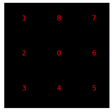
盤面を2次元プロットします。
# 盤面の状態を可視化する
def plot_puzzle(state = [0,1,0,1,1,1,1,0,0]):
    state_matrix = np.array(state).reshape(3,3)
    plt.imshow(state_matrix, cmap='gray', interpolation='none')
    for i in range(3):
        for j in range(3):
            pos = (i,j)
#             print(pos)
            button_num = DF.query("matrix_index==@pos")["button_num"].values[0]
#             print(button_num)
            plt.text(x=i,y=j,s=str(button_num),color='r',fontsize=18)
    plt.xlim([-0.5,2.5])
    plt.ylim([-0.5,2.5])
    plt.xticks([])
    plt.yticks([])
    plt.show()

メイン関数です。
initial stateを指定しているところしか違いません。
なお、Diffuserにおいて、このinitial state preparationをuncomputeする必要はありませんので、Grover部分は変わりません。
# 量子ビット数と古典ビット数
n = 9 #ボタンの数
q = 2 * n #量子ビット数. 2倍なのはボタン操作用に記録するビットがそれぞれあるから
c = 9 #古典ビット数
initial_state = [0,0,0,0,0,0,0,0,0] # 9-elements list consits of 0 or 1.
# initial_state = [0,0,1,0,1,0,1,0,1] # 9-elements list consits of 0 or 1.

# 最初に全ての状態(input)を同じ確率で重ね合わせる
circ_init = QuantumCircuit(q, c)
circ_init.h(range(n))

# 状態(state)をset
state_preparation(circ_init, initial_state = initial_state)
続きを前述の参考記事通りに実行して、得られた結果から盤面を計算します。
button_str = sorted_counts_sim[0][0] # most frequent bit pattern
state = calc_button_state(initial_state=initial_state, button_str=button_str)
print(state)
`[0, 0, 0, 0, 0, 0, 0, 0, 0]
となりました。
つまり、確かに量子アルゴリズムで得られた手順をやれば、盤面は一色(解状態)になります。
可視化しておきます。
plot_puzzle(state)
初期状態を変えてみる
initial_state = [0,1,1,0,0,0,1,0,1]

でやってみます。

これも解けました。
正しく実装できています。
解でない状態
Groverアルゴリズムにおいて、解が100%の確率で得られるとは限りません。
Groverアルゴリズムは、整数回の反復で解を増幅するのですが、整数であるがゆえに、ちょうど100%で狙って止めることは一般には出来ません。
例えばGroverアルゴリズムの実際の出力は、
[('010100110', 8186), ('110111011', 2), ('100010010', 1), ('100101100', 1), ('100010110', 1), ('100100010', 1)]
のように、解でない状態も一部得られます。
これらはどのような盤面に対応しているでしょうか。
「あと1手で解であるような、惜しい手順」だと思いますか?
実際に可視化してみます。


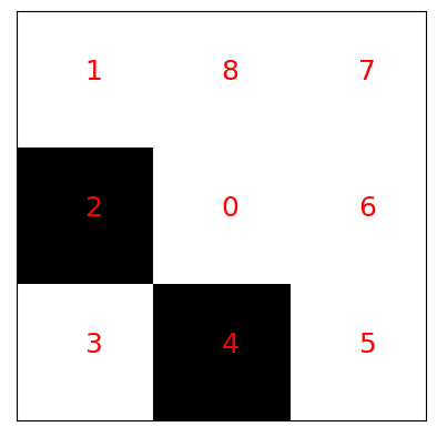
別にそういうわけではない ということがわかりますね。
Groverアルゴリズムは、解と解でない状態をTrueかFalseかで区別しているイメージになるので、解でない状態達は、それが解に”近い”か”遠い”かによらず、等しい確率で残っています。
これは原理的な話です。
でも、もし解に近い状態も回収したい(成功率を上げたい)と思ったら?
オラクル(解であることを定義する条件)を緩和するか、「解との”距離”(ハミング距離?)という数値を考慮する修正Groverアルゴリズム」を考えればよさそうですね。
そういう研究はすでにあるのではないかと思います。
やりすぎると、QAOAになりますね。
結論
今回は、QiitaにあったGroverアルゴリズムの記事を引用して、少し付加価値をつけてみました。
Groverアルゴリズムの実例はまだまだQiitaにも数少ないので、増やしていけたらと思います。